Accessibility Profiles

Measuring Vulnerability and Amendability of Transportation Network

Wojciech Pomianowski

Institute of Geography and Spatial Organization, Polish Academy of Sciences, Warszawa, Poland

1 STATE OF THE ART

Gravity and potential-based models have a long

standing tradition in geographic studies of

interactions. With the incorporation of graph data

structures, these models have undergone a

substantial improvement in terms of distance (or

generalised cost) component, which can be

calculated with realistic accuracy and with account

for real-life transportation network issues. Combined

graph-potential models are primary tool in two

domains: transportation studies and geography, with

the focus on slightly different questions. The

former’s interest is mostly in traffic volume, its

variability and correlation to areal units assigned as

origin and destination (Erlander and Stewart, 1990).

Models have been developed starting from pioneer

Chicago Area Transportation Study (CATS, 1960)

and nowadays highly sophisticated software tools

are available commercially (e.g. PTV 2013).

In the context of geography, the focus is less on

exact volume of flows and more on the impact of

transportation on territory, its population and

economy. One of the key concepts here is

accessibility – the “potential of opportunities for

interaction”, as originally formulated by Hansen

(1959), which can be re-stated as the ability of

certain place to provide good transportation for its

inhabitants and businesses (or, alternatively, the

property of a place to be easily accessed by the

outside inhabitants or businesses). Measures of

potential-based accessibility invariably stem from

potential formula (Isard W., 1960, owing to earlier

work of J.Q. Stewart):















(1)

where i-th point in space receives a sum of

influences of all other objects (indexed by j) of the

analysed system. Each influence is proportional to

the “mass” m

of a remote object and inversely

proportional to the distance to this object. To express

diminishing effect of distance on interaction, many

different functional forms have been employed

(Taylor, 1971) and this component is usually

elaborated separately under the name of distance-

decay function or impedance function. Except for

power function with negative β parameter, like

above, the exponent function exp (-βd

) is widely

used today.

Contemporary general formula (e.g. Geurs and

Ritsema van Eck, 2001)

















(2)

replaces distance with a generalized cost notion,

where travel time, distance or monetary cost can be

substituted. Accessibility of i-th object in a system is

a sum of influences of all other objects (indexed by

j). Each influence is a product of D

(j-th object

attractiveness) and c

– the cost of travel between i

and j reduced by distance decay function F.

Depending on study objective, many variables may

be used as attractiveness, from specific like

healthcare provision indices to general like

population or GDP.

Accessibility gives much better insight into

transportation network role in socio-economic

system then other measures like gross infrastructure

density indices (e.g. road density), or isochrone

surfaces (op cit.). Compared to first group, it does

relate the demand for travel to the supply of

infrastructure and even particular topology of

infrastructure. Compared to second, it does

incorporate distance decay concept and accounts for

all possible travel destinations (or origins). Also, it

has the property of additiveness, so values obtained

for singular objects may be legitimately aggregated

to wider areal units or the whole system (country) by

simple or weighted summation.

A notable feature of potential-based accessibility

is that it does, like no other measure, answer the

question of quality of the transportation system and

it does it in most direct way. In contrast to some

other policy-related terms like sustainability or

equity, the logic of accessibility computation is close

to commonsense semantics and the meaning is

Pomianowski, W.

Accessibility Proﬁles - Measuring Vulnerability and Amendability of Transportation Network.

In Doctoral Consortium (DCGISTAM 2016), pages 20-24

unequivocal – high accessibility is good, low is bad.

Thus, potential-based accessibility is a perfect

candidate for strategic goal setting, a benchmark or

evaluation criterion. Possibly, it can be tied to

investment effectiveness appraisal.

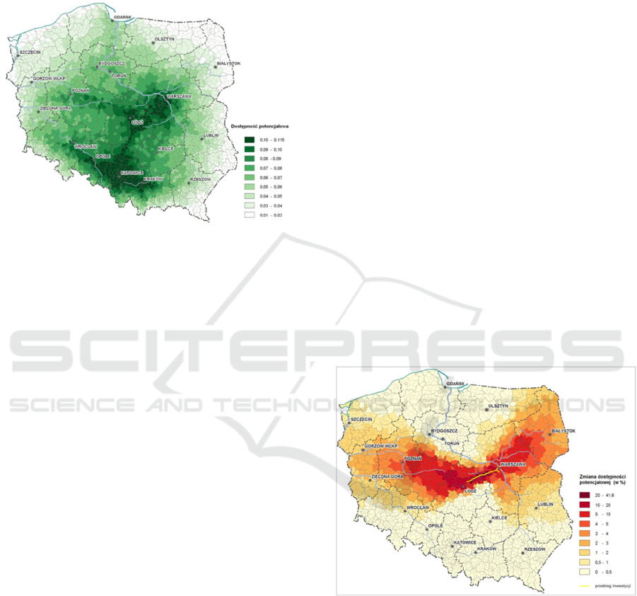
Figure 1: An example of potential-based accessibility in

road transportation. Source: IGiPZ website.

Starting in 2008, Ministry of Regional

Development of Poland become interested in a

methodological advances and a software tool

capable of evaluating the effects of EU-funded

transportation investments. The task was

accomplished with the help of tailor-made software

for graph-based potential accessibility computation.

Shortly after, the next software system OGAM –

Open Graph Accessibility Model (Pomianowski,

2012) was developed with significantly extended

architecture and features. The system accepts

arbitrary graph data set in ESRI shapefile format and

allows for formula-based specification of 1)

attracting masses, 2) velocity engine and 3) distance

decay function. Travel speeds are calculated

according to velocity engine specification and used

to assign the travel times to graph edges. Then a

shortest path algorithm finds the paths for every

node-node pair. O-D (origin-destination) matrix

found this way is fed into potential calculations. This

approach assumes that a transportation network is

unsaturated (no alternative paths or traffic load), so

the model is applicable only to regional or

countrywide level. Total accessibility is computed

with weighting, an extra feature is addition of self-

potential (see Appendix for explanations).

The most frequently used data and parameter set

used in OGAM was designed for private car road

transportation modeling and will be referred to as

OGAM Base Model. OGAM Base Model for

December 2014 is comprised of a network of 14400

edges of total length of 65525 km and 2321 nodes

corresponding to municipality administrative units

(LAU-2) plus 8884 auxiliary nodes (joins,

crossings). An attraction mass variable is census

population, which also serves as a weighting factor

for total (countrywide) accessibility computation.

Two exponential distance decay functions are in use,

with β parameter of 0.023105 for so called short

trips (everyday activity including commuting) with

mean of 30 min and 0.005775 for long trips

(business, leisure) with mean of 120 min. Travel

cost variable is equal to the travel time and is

derived from edge length and travel velocity. Travel

velocity is based on three factors: road category,

road inclination and surrounding population density,

combined by a

minimum()

function.

2 RESEARCH PROBLEM

OGAM system has been subsequently used in a

series of projects with different networks and

parameters. A lot of activity is directed towards

tracking accessibility improvement resulting from

adding new sections to ever increasing network of

motorways in Poland or upgrades made to existing

roads (e.g. Rosik and Stepniak, 2013).

Figure 2: Accessibility change after Warszawa-Lodz

motorway construction. Source: IGiPZ website.

The system performs well, giving numerical

results for pre-change and post-change state of

accessibility, which are then imported into GIS and

used for map production.

Individual simulations give good view of

particular event in network’s lifetime and reveal

some truth about the role of single edge or group of

edges in network connectivity. The scheme is as

follows: a change in edge’s travel cost (time) gives a

Accessibility Proﬁles - Measuring Vulnerability and Amendability of Transportation Network

response in accessibility measure, both locally (for

individual network nodes) and globally.

However, the results lack generality. We are able

to test a single improvement by changing a travel

time, but we may suspect that other, untested

changes on the analysed edge yield different and

unexpected changes in accessibility. Though the

monotonic relation between travel time and

accessibility seems to be beyond discussion, the

exact magnitude and shape of this relation in

different parts of the network is unexplored. Also, in

the current practice, only positive changes have been

tested, but exactly the same procedure could be used

to simulate negative changes. What is needed is

general characteristics of a network edge over the

whole range of travel time variability. With fixed

edge length this translates to the range of travel

speeds. Due to complex formulation and graph

involvement, no analytic solution exists to simply

derive a range of accessibility values from a single,

base value. The only solution is numerical simulation.

In above circumstances, a strong, unifying

concept was necessary and it appeared as a

accessibility response profile (explained in

METHODOLOGY section). The other need is of

technical nature: existing OGAM software was not

designed to run multiple simulations in a systematic

way because the complete dataset must be modified

and model must be run again for each simulation.

3 METHODOLOGY

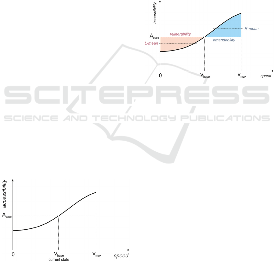
Figure 3 illustrates the concept of accessibility

response profile. X-axis runs along speed dimension,

from 0 value (no traffic) up to maximum allowed

speed (in case of Polish Traffic Code, 130 km/h). A

special point v

base

corresponds to actual, current

Figure 3: Generic accessibility response profile (exact

shape irrelevant).

value of speed on the link in the base model. Y-axis

runs along accessibility dimension. A special point

base

is actual, current value of accessibility

computed in the base model. A generic profile runs

from zero speed to maximum speed with ever

increasing A value and always crosses v

base

position.

Two parts of the profile may be distinguished

(see Figure 4): left part corresponds to negative

change usually related to congestion, accident

blocking, construction works or even complete

exclusion from traffic. This is the vulnerability area.

The bigger the area, the worse traffic disruption

occurs in case of negative event.

Figure 4: Profile functional structure.

The right part corresponds to improvements

resulting in increased speed due to construction (e.g.

surface or width improvement) or regulatory action

(higher speed limit, vehicle-type restrictions). This is

the amendability area. The bigger the are, the better

results may be achieved. A base point is neutral and

corresponds to current state of affairs. Please note,

that this “attachment” point for the profile is actually

not located in the middle, but on the right side for a

good road or left side for poor road. Thus, low speed

segments have small vulnerability area and cannot

do much harm to the network in case of failure. High

speed segments have small amendability area and

cannot give much improvement (in many cases they

have no amendability area at all).

Actual profiles given by series of simulations are

not smooth. They are approximated by nine speed

points, spread evenly across 0 – 130 km/h range.

Extra tenth value comes from the base model itself

and is computed once only. The test run results are

illustrated on Figure 5.

Observations on the shape, inclination and

attachment point give a complete information about

road segment’s importance and it’s influence on the

network. We may choose to observe the influence on

whole system or on particular node. This is why two

kinds of profiles will be computed:

DCGISTAM 2016 - Doctoral Consortium on Geographical Information Systems Theory, Applications and Management

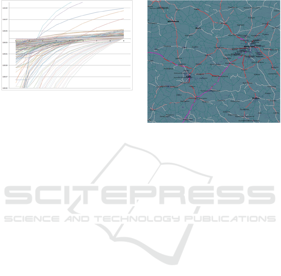
Figure 5: A sample of response profiles from test run.

• global profile with Y-axis describing the

accessibility response of the whole system,

and

• local profiles describing the accessibility

responses of a single nodes.

4 OBJECTIVES AND EXPECTED

OUTCOME

A series of descriptive and analytical procedures will

cover following topics:

1. Assessment of magnitude of influence across

segments (global accessibility).

2. Assessment of profile shapes and

categorization.

3. Ranking of segments according to global

influence, with mapping.

4. Mapping of global vulnerability and

amendability (see Figure 6 and Figure 7 for

preliminary maps).

5. Comparing global vulnerability and

amendability, seeking and summarizing

coincidences and differences.

6. Exploring the “foot” shaped profile

phenomenon (see Figure 5), which suggests a

redundancy of connectivity.

7. Comparing local accessibility magnitudes with

global effects.

8. Observing the relation of high-impact segments

to high-traffic segments. Challenging the thesis

that these always coincide (evidence exists).

9. Observing and quantifying the distance

between high-impact segment and it’s target

node (the node being influenced), based on

local accessibility. Supporting the thesis on far-

reaching influence.

Figure 6: Vulnerability (L-mean) map of road segments.

4.1 Challenges

Data Volume

Major objective of the first phase of analysis is

taming the sheer volume of data. Simulation of

global accessibility response brings 14400 profiles.

Simulations of local (node-related) accessibility

brings another 2321⨯ 14400 = over 33 million

profiles. Each profile is composed of 10 values. An

analysis should keep the profile data as a series and

not a unordered set or independent dimensions.

Time series analysis tools seem to be inappropriate

because the length of a series is limited.

Synthetic Measures

Two kinds of measures are necessary: one capturing

the magnitude of accessibility change, the other –

the structure (shape) of the profile. So far, for testing

and demonstration purposes, two simple magnitude

measures were computed (see Figure 4): R-mean, a

mean of amendability area under the right side of the

profile and L-mean - a mean value of vulnerability

area above left side of the profile. These are not

capable of capturing the variability of the width of

the profile and probably will be dropped in favour of

integral-based (surface) measures.

Mapping

Very detailed structure of the network must be

preserved to distinguish objects and this precludes

varying line widths and use of symbols. Colour

alone does not give good readability, especially for

paper medium.

Accessibility Proﬁles - Measuring Vulnerability and Amendability of Transportation Network

Figure 7: Amendability (R-mean) map of road segments.

5 STAGE OF THE RESEARCH

New software – OGAM Lab – has been developed

to complement OGAM capabilities with massive

simulation. Both programs share code responsible

for core functionality (reading network data, model

specification, shortest path algorithm etc.). Currently

OGAM Lab performs two tasks, and these have been

already completed for proper 2014 data:

• computation of path matrices (14400 files

totalling 130GB of data)

• computation of accessibility cube: a data file

with dimensions: nodes x edges x no.

simulations = 2321 x 14400 x 10.

The architecture allows for seamless inclusion of

next jobs, and these will be focused on accessibility

cube analytics.

REFERENCES

CATS, 1960. Chicago Area Transportation Study Vol. I-

III. https://archive.org/details/chicagoareatrans01chic

(accessed 19.11.2014).

Erlander S., Stewart, N., 1990. The Gravity Model in

Transportation Analysis – Theory and Extensions.

VSP BV Utrecht.

Geurs, K.T., Ritsema van Eck, J.R., 2001. Accessibility

Measures: Review and Applications. RIVM Report

408505 006. National Institute of Public Health and

the Environment, Bilthoven.

IGiPZ Accessibility Website. Maps by Marcin Stepniak.

<http://www.igipz.pan.pl/accessibility/pl/mapy.html>

(accessed 2.03.2016).

Isard, W., 1960. Methods of Regional Analysis: an

Introduction to Regional Science. The Technology

Press MIT, John Wiley & Sons Inc., New York –

London.

Pomianowski, W., 2012. OGAM – Open Graph

Accessibility Model. <http://www.igipz.pan.pl/access

ibility/pl/ogam> (accessed 12.02.2016).

PTV, 2013. Visum 13 Fundamentals. PTV AG, Karlsruhe.

Rosik, P., Stepniak, M., 2013. Accessibility improvement,

territorial cohesion and spillovers: a multidimensional

evaluation of two motorway sections in Poland.

Journal of Transport Geography 31, pp.154–163.

Taylor, P., 1971. Distance Transformation and Distance

Decay Functions, Geographical Analysis Vol. 3, Issue

3, July 1971, p. 221-238.

APPENDIX

Total accessibility

Summary countrywide accessibility computed as a

weighted total of node’s values. The weighting

occurs by node population P

raw or fraction.















(3)

Self potential

Self potential that is a measure of extra interaction

occurring within a node. It is based on assumption

that a great deal of transportation activity is released

for very short trips, confined to immediate node

vicinity. As this activity occurs below model

resolution, it must be accounted for in special way.

Compared to formula (2), an extended formula

























(4)

includes the front term with c

– the mean internal

cost (time) of travel within a node. This variable is

provided externally and is based on administrative

unit size.

DCGISTAM 2016 - Doctoral Consortium on Geographical Information Systems Theory, Applications and Management