The Six-Variable Model

Context Modelling Enabling Systematic Reuse of Control Software

Nelufar Ulfat-Bunyadi, Rene Meis and Maritta Heisel

paluno - The Ruhr Institute for Software Technology, University of Duisburg-Essen, Essen, Germany

Keywords:

Four-Variable Model, Context, Context Modelling, Contextual Decision, Satisfaction Argument, Domain

Knowledge, Requirement, Speciﬁcation.

Abstract:

A control system usually consists of some control software as well as sensors and actuators to monitor and

control certain quantities in the environment. The context of the control software thus consists of the sensors

and actuators it uses and the environment. When starting development of the control software, its context

is often not predeﬁned or given. There are contextual decisions the developers can make (e.g. which sen-

sors/actuators/other systems to use). By means of these decisions, the context is deﬁned step by step. Existing

approaches (like the Four-Variable Model) call for documenting the environmental quantities (monitored,

controlled, input, and output variables) that are relevant after making these contextual decisions. The en-

vironmental quantities that have originally been relevant (i.e. before deciding which sensors/actuators/other

systems to use) are not documented. This results in problems when the software shall later on be reused in

another, slightly different setting (e.g. with additional sensors). Then, it is hard for developers to decide which

environmental quantities are still relevant for the software. In this paper, we suggest an extended version of the

Four-Variable Model, the Six-Variable Model, and, based on that, a context modelling method, that combines

existing approaches. The beneﬁt of our method is that the environmental quantities that are relevant before

and after decision making are documented as well as the contextual decisions themselves and the options that

were selectable. In this way, later reuse of the software is facilitated.

1 INTRODUCTION

A control system usually consists of the control soft-

ware as well as sensors and actuators for monitoring

and controlling the environment (Parnas and Madey,

1995). The context of the control software comprises

the sensors and actuators it uses as well as the envi-

ronment it monitors/controls by means of them (Jack-

son, 2001). So, context modelling refers to modelling

or documenting this context.

The famous Four-Variable Model was suggested

by Parnas and Madey in 1995 and focuses also on

control systems (Parnas and Madey, 1995). It deﬁnes

the content of software documentation. Software doc-

umentation consists of different types of documents

(e.g. System Design Document, Software Require-

ments Document). Parnas and Madey describe these

documents as representations of one or more math-

ematical relations. These relations exist between the

following four types of variables: monitored variables

m (environmental quantities that the software mon-

itors through input devices, e.g. sensors), controlled

variables c (environmental quantities that the software

controls through output devices, e.g. actuators), input

variables i (data items that the software needs as in-

put), and output variables o (quantities that the soft-

ware produces as output). These four variables are il-

lustrated in Figure 1 together with a train control soft-

ware as an example.

Software-to-be

Environment

Input devices

(e.g. sensors)

Output devices

(e.g. actuators)

Monitored variables

(e.g. train speed)

Input data

(e.g. measured

speed)

Controlled variables

(e.g. doorsClosed)

Output results

(e.g. doorsState)

Figure 1: Four-variable model as illustrated in (van Lam-

sweerde, 2009).

In case of the train control software, the physical

speed of the train is the monitored variable and the

measured speed is the input variable. The differentia-

tion is important because these two variables might be

different. Consider, for example, aquaplaning. In this

Ulfat-Bunyadi, N., Meis, R. and Heisel, M.

The Six-Variable Model - Context Modelling Enabling Systematic Reuse of Control Software.

DOI: 10.5220/0005944100150026

In Proceedings of the 11th Inter national Joint Conference on Software Technologies (ICSOFT 2016) - Volume 2: ICSOFT-PT, pages 15-26

ISBN: 978-989-758-194-6

case, the measured speed of the train might be lower

than the actual speed of the train. The measured speed

might even be 0 km/h although the train is actually

still moving. The same holds for output variables and

controlled variables. The output variable ‘doorsState’

might be set to ‘closed’ but it could still happen that

not all train doors are actually closed. However, as

we will show in the following, documenting only four

variables is insufﬁcient. There are actually six vari-

ables that need to be documented.

As an example, we consider Adaptive Cruise Con-

trol (ACC) software (Robert Bosch GmbH, 2003).

The main objective of the software is to maintain the

driver’s desired speed while keeping the safety dis-

tance to vehicles ahead. To identify vehicles ahead

that are driving on the same lane, the ACC soft-

ware needs to ‘know’ the speed, the distance, and

the lane of vehicles ahead. To gain this information,

the ACC software uses a long range radar sensor and

ESP (Electronic Stability Program) sensors. The long

range radar (LRR) detects vehicles ahead and pro-

vides information about their speed, distance, and lat-

eral offset. The ESP sensors measure wheel speed,

yaw rate, lateral acceleration, and steering wheel an-

gle of the ACC vehicle itself. The ACC software uses

all this data in the following way: Based on the data

from the ESP sensors, the ACC software calculates

the yaw rate corrected for offset. This value enables

the ACC software to predict the course of the ACC

vehicle. Based on the lateral offset of vehicles ahead

(provided by the LRR) and the predicted course of the

ACC vehicle, the ACC software calculates the course

offset of vehicles ahead. The course offset is the es-

timated relative position of the vehicle ahead. In this

way, the ACC software estimates whether a vehicle

ahead is driving on the same lane or not. Accord-

ing to the Four-Variable Model (Parnas and Madey,

1995), the input and monitored variables given in Ta-

ble 1 would be documented.

Table 1: Input and monitored variables for ACC example.

Sensor

Input variable Monitored

variable

LRR

speed, distance, lat-

eral offset of vehicles

ahead

speed, distance,

relative position

of vehicles ahead

ESP

wheel speed, yaw

rate, lateral accelera-

tion, steering wheel

angle of ACC vehicle

course of ACC

vehicle

In contrast to that, the variables that were actually

relevant (i.e. before making the decision to use the

long range radar and the ESP sensors) are: the speed,

the distance, and the lane of vehicles ahead as well as

the lane of the ACC vehicle. Yet, these are not doc-

umented. This situation results in problems when the

ACC software shall later on be reused in another set-

ting. Imagine that the ACC software shall later on

be reused in the next car generation. However, in

the next generation, the ACC vehicle is additionally

equipped with a stereo video sensor which provides

precise information about the lane of vehicles ahead

and the lane of the ACC vehicle. Having documented

only the information given in Table 1, it is quite hard

for developers to decide which input and monitored

variables are still necessary and which ones are not.

In summary, the context of the software-to-be is

not completely predeﬁned or given. Developers make

contextual decisions and thereby deﬁne the context

step by step. Existing approaches (like the Four-

Variable Model (Parnas and Madey, 1995) but also

others; see Section 5) only call for documenting the

variables that are relevant after decision-making, i.e.

the classical four variables. None of the approaches

calls for documenting the contextual decisions that

are made (together with the options that were se-

lectable) and the variables that have been relevant be-

fore decision-making. In this paper, we suggest a

context modelling method that ensures the documen-

tation of all this information. Our method is based

on an extended version of the Four-Variable Model

which we call the Six-Variable Model.

The paper is structured as follows. In Section 2,

we present some fundamental concepts that provide

the basis for our work. In Section 3, we introduce

our Six-Variable Model. Section 4 contains a descrip-

tion of our context modelling method which is based

on the Six-Variable Model and combines existing ap-

proaches. We discuss related work in Section 5 and

ﬁnally conclude our paper in Section 6.

2 FUNDAMENTALS

We use the terminology deﬁned by Zave and Jackson

(Zave and Jackson, 1997) and differentiate between

system, machine, and environment. A system consists

of manual and automatic components. The machine is

the computer-based artefact of the system that is the

target of software development. The environment is

a portion of the real world that is becoming the en-

vironment of the development project because its cur-

rent behaviour is unsatisfactory in some way. The ma-

chine will be inserted into the environment so that the

behaviour of the environment becomes satisfactory.

There are indicative and optative statements about

ICSOFT-PT 2016 - 11th International Conference on Software Paradigm Trends

the environment. Indicative statements describe the

environment as it is without or in spite of the ma-

chine. Optative statements describe the environment

as we would like it to be because of the machine.

Based on this differentiation, requirements, domain

knowledge, and speciﬁcation are deﬁned as follows.

A requirement is an optative statement, intended to

express the desires of the customer concerning the

software development project. Domain knowledge or

domain assumptions represent indicative statements

intended to be relevant to the software development

project. The speciﬁcation is an optative statement, in-

tended to be directly implementable and to support

satisfaction of the requirements. The relation between

the set of requirements (R), the set of domain knowl-

edge/assumptions (K), and the set of speciﬁcations

(S) is deﬁned by means of the satisfaction argument

given in Equation 1.

S, K ` R (1)

The satisfaction argument says that if a machine is

developed that satisﬁes S and is inserted into the en-

vironment as described by K, then the set of require-

ments R is satisﬁed.

3 OUR SIX-VARIABLE MODEL

We ﬁrst describe how we derived the Six-Variable

Model based on the Four-Variable Model (see Section

3.1). Then, we explain the notation that might be used

to document the six variables (see Section 3.2). Fi-

nally, we introduce four so called domain knowledge

frames that can be used to make assumptions that are

implicit in the Six-Variable Model explicit (see Sec-

tion 3.3).

3.1 Derivation of the Model

As explained above, Parnas and Madey (Parnas and

Madey, 1995) deﬁne not only the four variables (mon-

itored, controlled, input, and output) but also the fol-

lowing mathematical relations between them:

• NAT: indicative relation between m and c

• REQ: optative relation between m and c

• IN: indicative relation between m and i

• OUT: indicative relation between o and c

• SOF: optative relation between i and o

On the one hand, the environment (i.e. nature and

previously installed systems) places constraints on

the values of the environmental quantities m and c.

These are described by NAT. On the other hand,

the software-to-be is expected to impose further con-

straints on them. These are described by REQ. IN de-

scribes how sensors translate m to i. OUT describes

how actuators translate o to c. SOF, ﬁnally, describes

how the software-to-be will/shall produce its output o

from the input i.

As explained in the introduction, we argue that

documenting only the classical four variables is in-

sufﬁcient. The four variables result from the decision

which sensors/actuators/other systems to use for mon-

itoring/controlling quantities in the environment. The

quantities that were originally relevant in the require-

ment are often different than the ones that are ﬁnally

monitored/controlled. In the ACC example, the lane,

speed, and distance of vehicles ahead as well as the

lane of the ACC vehicle were environmental quan-

tities that were originally relevant. Yet, due to the

decision to use a long range radar and ESP sensors

for monitoring, other environmental quantities were

monitored: the relative position, speed, and distance

of vehicles ahead as well as the course of the ACC ve-

hicle. Therefore, we extend the Four-Variable Model

with the following two variables:

• referenced variable r: environmental quantities

that should originally be observed/monitored and

were therefore referenced in the requirement

• desired variable d: environmental quantities that

should originally be inﬂuenced and that shall be

as desired by the requirement

The introduction of the two new variables necessitates

that the following mathematical relations between the

variables are described as well:

• IN

: indicative relation between r and m

• OU T

: indicative relation between c and d

• NAT

: indicative relation between r and d

• REQ

: optative relation between r and d

describes how a referenced variable is related to

a monitored one (e.g. how lane of vehicles ahead is

related to relative position of vehicles ahead). Note

that there does not necessarily need to be a 1-to-1

mapping between the variables. Actually, lane of ve-

hicles ahead is not only related to relative position of

vehicles ahead but also to course of the ACC vehicle,

since both are used to estimate the lane of vehicles

ahead. So, there may be a 1-to-n, n-to-1, n-to-m map-

ping between r and m variables. Similarly, OUT

describes how controlled variables are related to de-

sired variables. Beyond that, there is an indicative

and an optative relation between the newly introduced

r and d variables. These are documented by means of

the relations NAT

and REQ

. We will explain

these relations later on in more detail.

The Six-Variable Model - Context Modelling Enabling Systematic Reuse of Control Software

3.2 Documentation of the Six Variables

For documenting the six variables, Jackson’s prob-

lem diagrams (Jackson, 2001) are well suited. Jack-

son differentiates between the world (i.e. the environ-

ment) and the machine (i.e. the software-to-be). The

software development problem to be solved is in the

real world, the environment. The machine is inserted

into this environment to solve the problem. In prob-

lem diagrams, the machine and its connection to the

problem/requirement in the real world can be mod-

elled in terms of so called problem domains that are

in between. The six variables can also be made ex-

plicit: they can be documented as phenomena at the

different types of connections between the domains.

We ﬁrst introduce the notation and then explain the

documentation of the six variables in more detail.

According to Jackson’s method (Jackson, 2001),

ﬁrst, a context diagram is created showing the ma-

chine in its environment. Then, the overall software

development problem is decomposed into subprob-

lems, and each subproblem is documented in a prob-

lem diagram. As a support in creating problem di-

agrams, Jackson provides so called problem frames,

which are patterns of recurring software development

problems. They are intended to be used when decom-

posing software development problems by instantiat-

ing them.

A context diagram consists of the following mod-

elling elements: the machine domain (representing

the software-to-be), usually several problem domains

(representing any material or immaterial object in the

environment, e.g. people, other systems, a physical

representation of data), and interfaces (of shared phe-

nomena, e.g. events, states, values) connecting the

machine domain and problem domains. At the inter-

face, not only the phenomena are annotated but also

the abbreviation of the domain controlling the phe-

nomena followed by an exclamation mark (e.g. M!).

The other domain that participates in the interface ob-

serves these phenomena. An example of a context

diagram is given in Figure 11.

Additionally to the elements of a context diagram,

a problem diagram contains a requirement, a con-

straining reference, and optionally one or more re-

quirement references. A requirement reference con-

nects the requirement and a problem domain express-

ing that the requirement refers somehow to the do-

main phenomena. A constraining reference connects

also the requirement and a problem domain, but ex-

presses that the requirement not only refers to but

even constrains the domain phenomena. An example

of a problem diagram is given in Figure 12.

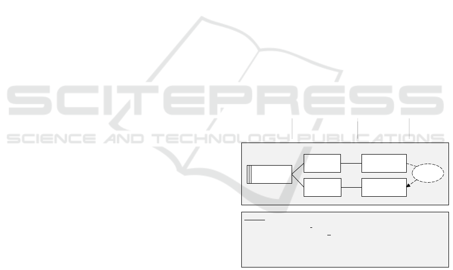
In Figure 2, we have depicted the Six-Variable

Model itself as a problem diagram. The software-

to-be is the control machine. Sensors and actuators

are used by the machine to monitor/control the envi-

ronmental domains W and Z. Jackson calls the sen-

sors and actuators connection domains. A connec-

tion domain is a domain that is interposed between

the machine and a problem domain (Jackson, 2001).

There are reliable and unreliable connection domains.

According to Jackson, they shall only be modelled

if they are unreliable. If they are reliable, they can

be omitted in the problem diagram. As regards our

Six-Variable Model, note that there are maybe sev-

eral connection domains (i.e. a chain of sensors or a

chain of actuators) between the machine and the en-

vironment, especially in embedded systems. For an

example, consider again the ACC system described

above. The driver may press the brake pedal to de-

activate ACC. Yet the brake pedal is not directly con-

nected to the ACC. The brake pedal is connected to

two sensors: a travel sensor and a pressure sensor to

measure the speed and force of the driver’s command.

These sensors are connected to the ESP and the ESP

is connected to the ACC. The existence of connection

domains means that there are not only six variables to

be documented but even 4 + n variables. However, the

method we present in this paper is already designed to

consider the case that there may be more connection

domains (see Section 4).

Control

machine

Environmental

domain W

Require-

ment

Environmental

domain Z

SE!i

CM!o

Sensors

EW!m

EW!r

Actuators

EZ!d

AC!c

Legend:

r: variables originally referenced by the requirement

d: variables that shall be as desired by the requirement

m: variables actually monitored by sensors

c: variables actually controlled by actuators

i: input variables

o: output variables

Sensors/actuators/other

systems connecting

software-to-be to real world

Requirement

in real world

Software-to-be

Remote problem

domains

in real world

Figure 2: Our Six-Variable Model.

The mathematical relations between the six variables

are depicted in Figure 3. We have renamed the re-

quirement to be satisﬁed in the real world as RW-

Req. Furthermore, we added two requirements: Sof-

Req (the set of software requirements) and Sys-Req

(the set of system requirements). Sof-Req is actu-

ally the speciﬁcation SOF expressing how i is trans-

formed into o. The system consists of the software

(the machine) and the sensors and actuators. There-

fore, Sys-Req represents the set of system require-

ments and refers to m while constraining c. RW-Req

ICSOFT-PT 2016 - 11th International Conference on Software Paradigm Trends

refers to r and constrains d. SOF, REQ, and REQ

are optative. The corresponding indicative relations

between m and c as well as r and d are described by

NAT and NAT

. Further indicative relations are IN,

, OUT, and OUT

Sensors/actuators/other

systems

Requirement

in real world

Software-to-be

Remote problem

domains in real world

Control

machine

Environmental

domain W

Environmental

domain Z

Sensors

Actuators

OUT

Sof-Req

= SOF

Sys-Req

= REQ

NAT

RW-Req

= REQ

Figure 3: Relations among six variables.

3.3 Assumptions in the Six-Variable

Model

According to Parnas and Madey, IN and OUT are

indicative relations (Parnas and Madey, 1995). Yet,

in our opinion, IN and OUT as well as IN

and

OUT

can also be considered to be optative. We

want these relations to be true, but they are not really

facts. Rather, they are assumptions. Van Lamsweerde

(van Lamsweerde, 2009) makes an interesting differ-

entiation. He considers three types of domain knowl-

edge: domain properties, domain hypotheses, and ex-

pectations. Domain properties are descriptive state-

ments about the environment and are facts (e.g. phys-

ical laws). Domain hypotheses are also descriptive

statements about the environment, but are assump-

tions. Expectations are also assumptions, but they are

prescriptive statements to be satisﬁed by environmen-

tal agents like persons, sensors, actuators. We adopt

van Lamsweerde’s three types of domain knowledge

and suggest four domain knowledge frames which

can be used to make the expectations and domain hy-

potheses in the Six-Variable Model explicit. The do-

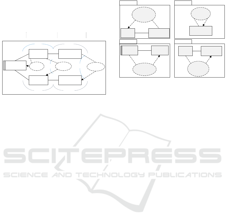
main knowledge frames are given in Figure 4. Each

frame can be instantiated to create the corresponding

domain knowledge diagram. Domain knowledge di-

agrams have already been introduced in (Alebrahim

et al., 2014). However, the four domain knowledge

frames we present here are new. The beneﬁt of mak-

ing domain hypotheses and expectations explicit is

that (i) the developers of the machine become aware

of them and (ii) the expectations can be discussed

with the developers or providers of these sensors, ac-

tuators, and other systems and, thus, be reviewed by

them.

Environmental

domain Z

Actuator

AC!c

Exp: d is

actually

achieved by

EZ!d

AC!c

Frame 4

Environmental

domain W

DH: m

actually

reflects r

EW!r

EW!m

Environmental

domain W

Sensors

EW!m

Exp: i

actually

corresponds

to m

SE!i EW!m

Control

machine

CM!o

Actuator

Exp: o

actually

results in c

CM!o AC!c

Frame 1

Frame 2

Frame 3

Figure 4: Domain knowledge frames.

Frame 1 in Figure 4 expresses that there is a domain

hypothesis about the domain W which says that m ac-

tually reﬂects r. This is a domain hypothesis made

by us (as the developers of the machine). Frame 2

expresses that there is an expectation to be satisﬁed

by the sensor domain. The sensor domain has to en-

sure that i actually corresponds to m. Frame 3 ex-

presses that there is an expectation to be satisﬁed by

the actuator domain. The actuator domain has to en-

sure that o actually results in c. Finally, frame 4 ex-

presses that there is an expectation to be satisﬁed by

the controlled domain Z. Domain Z is responsible for

ensuring that d is actually achieved by c. Note that we

have a domain hypothesis in Frame 1 while Frames 2

to 4 present expectations. All four statements are as-

sumptions. Yet, the difference lies in the prescriptive

and descriptive character of the statements. In Frames

2 to 4, we make prescriptions for certain domains: for

the sensor (Frame 2), the actuator (Frame 3), and the

controlled domain (Frame 4). They are responsible

for coming up to our expectations. Yet, in Frame 1,

we cannot make domain W responsible for satisfy-

ing our assumption. It is rather a hypothesis we make

which needs to hold.

4 CONTEXT MODELLING

In this section, we present a method that is based on

the Six-Variable Model and supports developers in

documenting not only the six variables but also the

contextual decisions that are made as well as the op-

tions that were selectable. We explain the techniques

we use and the reason why we chose them in Section

4.1. Afterwards, we present the method steps in Sec-

tion 4.2. The application example is described in Sec-

tion 4.3. Finally, we explain the beneﬁt of the created

models in Section 4.4.

The Six-Variable Model - Context Modelling Enabling Systematic Reuse of Control Software

4.1 Used Techniques

Problem Diagrams. As described in Section 3, prob-

lem diagrams (Jackson, 2001) are well suited for

modelling the six variables, since they show the re-

quirement, the remote problem domains, the connec-

tion domains, and the machine domain in one diagram

together with the shared phenomena. Yet, develop-

ers need guidance in documenting the ‘right’ six vari-

ables therein and not other phenomena. We provide

this guidance in our method (see Section 4.2). Al-

though we use problem diagrams, we do not proceed

in the way suggested by Jackson during problem de-

composition. Our method proceeds in another way.

For creating the problem diagrams, we used the

UML4PF tool (Cote et al., 2011). The beneﬁt of us-

ing this tool is that different other analyses can be per-

formed on the models that are created with this tool.

In UML4PF, problem diagrams are shown as UML

class diagrams with corresponding stereotypes to ex-

press the semantics of problem diagram model ele-

ments. For more details regarding the mapping of the

notations, see (Cote et al., 2011).

Differentiating between Essence and Incarnation.

The differentiation between essence and incarnation

of a system was introduced 1984 by McMenamin and

Palmer (McMenamin and Palmer, 1984). The essence

comprises the capabilities that a system must pos-

sess to fulﬁl its purpose, regardless of how the sys-

tem is implemented. The incarnation comprises all

implementation details. A heuristic for identifying

the essence of a system is the assumption of perfect

technology, i.e. the assumption that the technology

within the system is perfect, i.e. processors are, for

example, able to do anything constantly and contain-

ers are able to hold an inﬁnite amount of data. We

use the differentiation between essence and incarna-

tion in our method too. Yet, to identify the essence,

we assume that the technology outside the machine

is perfect. This means, for example, that connec-

tion domains like sensors and actuators are consid-

ered to be reliable and are therefore not shown in the

corresponding context/problem diagram. To consider

the incarnation, the assumption of perfect machine-

external technology is then given up.

OVM and Selection Model. To document con-

textual decisions and options/alternatives, we use the

OVM (Orthogonal Variability Model) (Pohl, 2010).

The OVM was originally developed to capture the

variation points and variants of a product line together

with their variability dependencies (mandatory, op-

tional, alternative choice) as well as constraint depen-

dencies (requires, excludes). The variants can be re-

lated to a development artefact like a requirement or

a diagram (or a part of it) by means of so called arte-

fact dependencies. The artefact (or the part of it) is

then deﬁned as being variable. For documenting the

choices that are made, a selection model is created.

We use the OVM to document the contextual deci-

sions to be made, the options/alternatives that are se-

lectable, and dependencies among them. By means

of artefact dependencies, we relate the alternatives

to variable elements of the AND/OR graph (see next

section). To document the choices, we also use a se-

lection model. The strength of the OVM and the main

reason for choosing this approach over others is that

one is able to relate a variant to an entire model, a

model element, or even certain sections of a model.

AND/OR Graph. For documenting the reﬁne-

ment/decomposition of requirements, we use an

AND/OR graph (which is similar to the AND/OR

goal graph described in (Pohl, 2010)). The AND/OR

graph is a directed, acyclic graph with nodes that rep-

resent requirements and edges that represent AND-

decomposition relationships and OR-decomposition

relationships between the requirements. A decom-

position of a requirement R into a set of subrequire-

ments R

,..., R

is an AND-decomposition iff all sub-

requirements must be satisﬁed to satisfy the require-

ment R. A decomposition of a requirement R into a set

of subrequirements R

,..., R

is an OR-decomposition

iff satisfying one of the subrequirements is sufﬁcient

for satisfying the requirement R. What needs to be

documented in addition to the AND/OR graph, is the

reasoning why each AND/OR-decomposition is suf-

ﬁcient. We suggest documenting this information at

least informally in natural language.

4.2 Method Steps

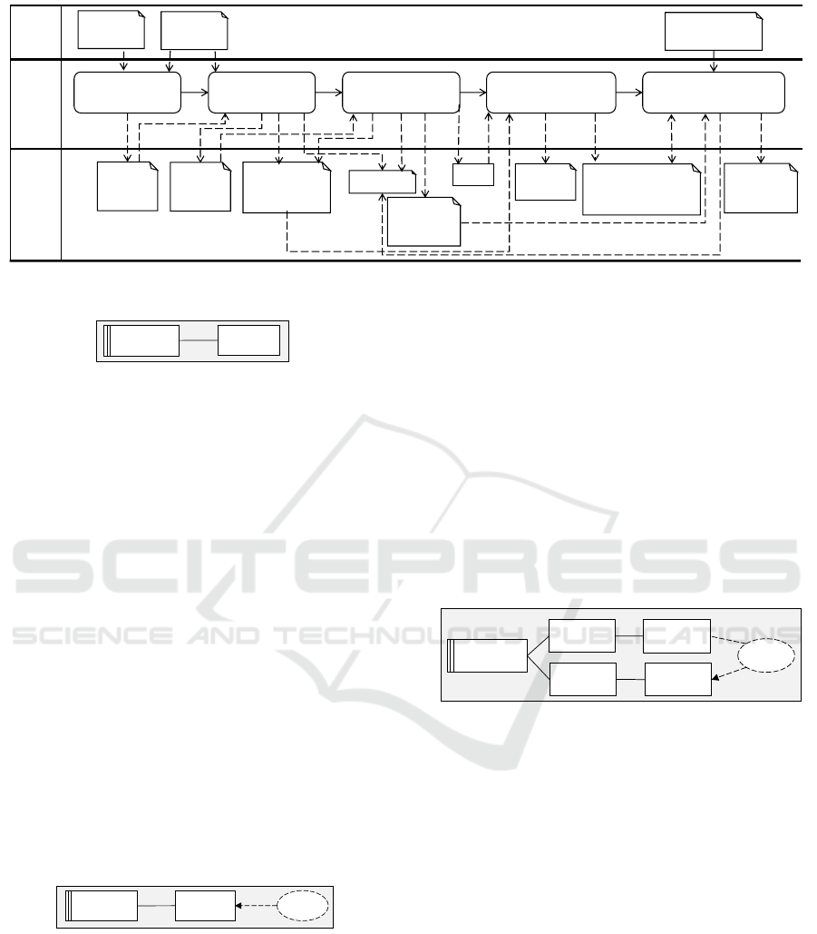
Figure 5 provides an overview of the method steps as

well as the input and output of each step.

Step 1: Create an essential context diagram. As

a ﬁrst step, the remote problem domains are identi-

ﬁed and a context diagram showing the machine do-

main, the remote problem domains, and the interface

between them with the r and d variables is created

(see Figure 6). The context diagram is essential, since

we assume that the connection domains are all reli-

able and, thus, abstract from them. As input to Step

1, knowledge about the machine and its environment

is needed.

Step 2: Create essential problem diagrams. Dur-

ing this step, the overall problem/requirement is de-

composed/reﬁned and, for each requirement, an es-

sential problem diagram is created. The informa-

tion to be documented in an essential problem dia-

gram is given in Figure 7. An essential problem dia-

ICSOFT-PT 2016 - 11th International Conference on Software Paradigm Trends

external

input

method

steps

input

output

Step 1:

Create essential

context diagram

Step 2:

Create essential

problem diagrams

Step 3:

Create incarnation

problem diagrams

Step 4:

Select alternatives and

derive concrete model

Step 5: Make

expectations and domain

hypotheses explicit

Essential

context

diagram

AND/OR graph

with all

alternatives

Reasonings

Selection

model

Domain

knowledge

diagrams

Essential

problem

diagrams

OVM

Incarnation

problem

diagrams

Derived AND/OR

graph with

selected alternatives

Domain

knowledge frames

Domain

expertise

Six-Variable

Model

Figure 5: Overview of our context modelling method.

Control

machine

Remote

domains

r, d

Figure 6: Information to be documented in an essential con-

text diagram.

gram shows the machine (or more precisely the sub-

machine), the remote problem domains, the require-

ment, interfaces between machine and remote prob-

lem domains annotated with r and d variables as well

as requirement references and constraining references

annotated with r and d variables. Through the re-

ﬁnement/decomposition of the requirement, the prob-

lem domains that were shown in the context diagram

may also be decomposed into several ones. So it

may be the case that the problem diagrams contain

the decomposed problem domains. This is allowed

as long it is ensured that all problem domains shown

in the problem diagrams are either shown as well in

the context diagram or represent parts of the problem

domains shown therein. The decomposition of the

overall problem/requirement may be done in several

steps, if necessary. The decomposition relationships

of the problems/requirements are documented as an

AND/OR graph. For each AND/OR decomposition

of a requirement, the reasoning why the decomposi-

tion is sufﬁcient is documented too.

Control

machine

Remote

domains

REQ

r, d

Figure 7: Information to be documented in an essential

problem diagram.

Step 3: Create Incarnation Problem Diagrams.

For each essential problem diagram from Step 2, con-

nection domains (if existent) are added and thus in-

carnation problem diagrams are created. If there

are different options/alternatives for using certain

sensors/actuators (i.e. connection domains), create

separate incarnation problem diagrams for each op-

tion/alternative. Figure 8 shows which information

needs to be documented in an incarnation problem di-

agram. The main difference is that sensors and ac-

tuators are considered and, thus, the m, c, i, o vari-

ables are introduced. If there are options/alternatives,

a decision point with the corresponding alternatives

is also created in an OVM. Due to the new require-

ment decompositions, the AND/OR graph from Step

2 needs to be extended and corresponding reasonings

need to be created. The decision points and alter-

natives in the OVM are related to the corresponding

variable elements of the AND/OR graph by means of

artefact dependencies.

Control

machine

Monitored

remote

domains

REQ

Sensors

Actuators

Controlled

remote

domains

Figure 8: Information to be documented in an incarnation

problem diagram.

Step 4: Select Alternatives and Derive Concrete

Model. For each decision point in the OVM, one or

(if possible and appropriate) several alternatives are

selected. The choices are documented in a selec-

tion model. Based on the selection model, a concrete

model of the requirement decomposition is derived

from the AND/OR graph .

Step 5: Make Expectations and Domain Hypothe-

ses Explicit. To each incarnation problem diagram

that has been selected in Step 4, the four domain

knowledge frames (introduced in Section 3) are ap-

plied to make the domain hypotheses and expec-

tations explicit in separate domain knowledge dia-

grams. This results in a decomposition of the require-

ment from the incarnation problem diagram. We illus-

trate this in Figure 9. If the domain hypothesis DH is

valid, the expectations Exp-Se, Exp-Ac, and Exp-CD

are satisﬁed (by the sensors, actuators, and controlled

The Six-Variable Model - Context Modelling Enabling Systematic Reuse of Control Software

domains), and the machine satisﬁes its software re-

quirement Sof-Req, then the real world requirement

REQ

is satisﬁed (see satisfaction argument in Fig-

ure 9). The derived AND/OR graph from Step 4 is

extended with the requirement decompositions made

in this step. Thus, the satisfaction argument is also

reﬂected in the AND/OR graph. The reasoning for

these decompositions need to be documented as well.

DH: m

actually

reflects r

Control

machine

Monitored

remote

domains

REQ

Sensors

Actuators

Controlled

remote

domains

Exp-Se: i

actually

corresponds

to m

Exp-Ac: o

actually

results in c

Exp-CD: d is

actually

achieved by c

Sof-Req:

produce o

from i

Satisfaction argument: DH, Exp-Se, Sof-Req, Exp-Ac, Exp-CD ├ REQ

Figure 9: Progression towards the machine.

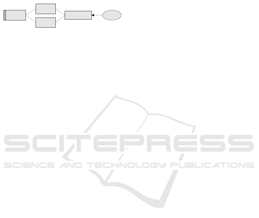
The application of the method results in a number

of models that are related to each other. The inter-

model relationships are depicted in Figure 10. Note

that only those concepts of the models are shown that

need to be related to each other. The relationships

between the OVM/selection model and the AND/OR

graph need to be documented as artefact dependen-

cies. The relationships between requirements in the

two AND/OR graphs (the one containing all alterna-

tives/options as well as the one containing only the

selected alternatives/options) and the requirements in

the problem diagrams need to be documented as well

by means of traceability relationships. The same

holds for the relationships between the domain hy-

potheses and expectations (both representing domain

knowledge) in the domain knowledge diagrams and

the problem diagrams to which they contribute.

4.3 Application to Real Example

We applied our method to a real example: the ACC

described in (Robert Bosch GmbH, 2003). Due to

Domain knowledge diagram

Problem diagram

OVM / Selection model

AND/OR graph

Variation point Variant

Requirement

Requirement Domain knowledge

◄ relates to

requires

satisfaction of ►

Domain hypothesis

Expectation

Fact Assumption

Figure 10: Inter-model relationships.

Figure 11: Essential context diagram for ACC example.

space limitations, we are not able to describe the en-

tire example here and show only excerpts.

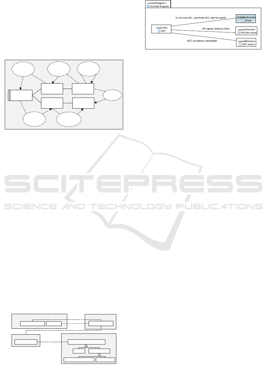
Step 1: Create an Essential Context Diagram. An

essential context diagram for the ACC example is

given in Figure 11. It shows three remote problem

domains in the real world: the driver, vehicles ahead,

and the ACC vehicle. Since we abstract from con-

nection domains, the ACC machine is directly con-

nected to these problem domains. The interfaces are

annotated with the environmental quantities of these

problem domains that we are interested (the r and d

variables).

Step 2: Create Essential Problem Diagrams.

The overall requirement R-0: “Maintain desired

speed keeping safety distance to vehicles ahead.” is

decomposed into the following requirements:

R-1: Enable driver to activate ACC.

R-2: Enable driver to enter desired speed.

R-3: Identify vehicles ahead for tracking.

R-4: Adapt speed to desired speed keeping safety

distance to vehicles ahead.

R-5: Display recorded desired speed to driver.

R-6: Enable driver to deactivate ACC.

The following reasoning explains why this decompo-

sition is sufﬁcient:

The decomposition into R-1 to R-6 is sufﬁcient

because: R-1 ensures that the ACC machine

enters the “activated” state while R-6 ensures

that the ACC machine leaves this state. In the

“activated” state, the machine is able to sat-

isfy R-2 to R-5 as follows. R-2 ensures that

the driver may enter a new desired speed if he

wants to. Otherwise, the ACC machine uses

the currently stored desired speed. R-3 en-

sures that the ACC machine detects vehicles

ahead driving on the same lane. R-4 ensures

that the ACC machine not only drives at the

desired speed but adapts the speed, if it detects

vehicles ahead. R-5 ensures that the driver is

always informed about the desired speed that

is currently stored and used by the ACC ma-

chine.

ICSOFT-PT 2016 - 11th International Conference on Software Paradigm Trends

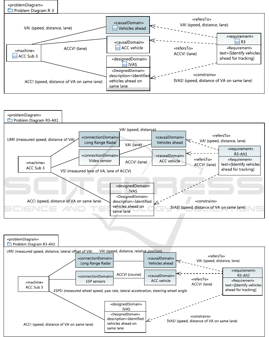
Figure 12: Essential problem diagram for R-3.

Figure 13: Incarnation problem diagram for R3-Alt1.

Figure 14: Incarnation problem diagram for R3-Alt2.

The essential problem diagram for R-3 is shown in

Figure 12. One peculiarity in Figure 12 is that we

introduced a designed domain called IVAS (identiﬁed

vehicles ahead on same lane). IVAS is a so called

The Six-Variable Model - Context Modelling Enabling Systematic Reuse of Control Software

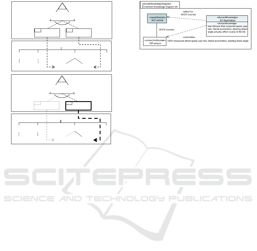
Identifying lane of

vehicles ahead

VPVP

Estimating

the lane

Using a

video sensor

OVM

AND/OR graph

R-0

R-1 R-2

R-3 …

R3-Alt1

R3-Alt2

[1…1]

R1-Alt1

R2-Alt1

Identifying lane of

vehicles ahead

VPVP

Estimating

the lane

Using a

video sensor

Selection model

AND/OR graph

R-0

R-1 R-2

R-3 …

R3-Alt1

R3-Alt2

[1…1]

R1-Alt1

R2-Alt1

Figure 15: Part of the OVM for the ACC Software.

designed domain, i.e. it is actually part of the machine

ACC Sub 3. Based on the information ACC Sub 3

gets, it decides whether detected vehicles ahead are

on the same lane or not. The ones that are on the

same lane are stored by ACC Sub 3.

Step 3: Create Incarnation Problem Diagrams.

Examples of incarnation problem diagrams are given

in Figures 13 and 14. These are two possible incar-

nations for the essential requirement R-3 (shown in

Figure 12). Alternative 2 represents the ACC system

as described in the introduction using ESP sensors

and the long range radar to identify vehicles ahead

for tracking. In Alternative 1, in contrast, the long

range radar is used together with a stereo video sen-

sor for the same purpose. In case of Alternative 1, the

lane of vehicles ahead is identiﬁed precisely, while it

is only estimated in case of Alternative 2. The r and

d variables (at the requirement reference and the con-

straining reference) in Figure 13 and Figure 14 are the

same, while the m, i, c, o variables at the interfaces are

different.

Step 4: Select Alternatives and Derive Concrete

Model. Figure 15 depicts an excerpt of the OVM with

the artefact dependencies (shown as dashed arrows) to

the AND/OR graph as well as a selection model and

the derived AND/OR graph. In the selection model

and the derived AND/OR graph, the alternatives that

are not selected are shown in grey (R3-Alt1) while the

selections are emphasized (R3-Alt2).

Step 5: Make Expectations and Domain Hypothe-

Figure 16: Example of a domain knowledge diagram.

ses Explicit. An example of a domain knowledge di-

agram (created by instantiating Frame 2) is given in

Figure 16. It shows the expectation we, as developers

of the ACC software have, regarding the ESP sensors

shown in Figure 14. This expectation is to be satisﬁed

by developers of the ESP sensors. We expect that the

wheel speed, yaw rate, lateral acceleration, and steer-

ing wheel angle measured by the ESP sensors actually

reﬂect the course of the ACC vehicle. Therefore, the

ESP sensors are constrained in the domain knowledge

diagram in Figure 16, while the ACC vehicle is refer-

enced.

4.4 Beneﬁt

The documentation that is created when applying our

method enables developers to analyse the impact of

contextual changes systematically and to integrate

changes in a consistent manner. For example, if the

ACC software shall actually be reused in another ve-

hicle that is additionally equipped with a video sensor,

the developers can see in the documentation what the

current r is in the problem diagram for R-3 (identi-

fying vehicles ahead) and how it is realized (m and

i). In the OVM, they can even see that there was a

decision point regarding lane identiﬁcation and that

a video sensor was even considered as an alternative.

As another example consider the case in which other

developers tell us that they are not able to provide the

input variable i we expected from them but a slightly

different one. Based on the documentation, we are

able to trace back to which r this variable contributed

and whether there are other alternatives to achieve r.

5 RELATED WORK

Jackson discusses the Four-Variable Model in his

book (Jackson, 2001) as well. He depicts the Four-

Variable Model as a problem diagram which is shown

in Figure 17. The machine is a control machine which

uses sensors and actuators to monitor/control the en-

vironment. The four variables are annotated at the in-

terfaces between machine, sensors/actuators, and en-

ICSOFT-PT 2016 - 11th International Conference on Software Paradigm Trends

vironment. The constraining reference (which is at

the same time also a requirement reference) is anno-

tated with the m and c variables which means that the

requirement REQ refers to the variable m and con-

strains the variable c of the environment.

Control

machine

Actuators

Sensors

SE!i

CM!o

Environment

EN!m

AC!c

REQ

m,c

Figure 17: Four Variable Model as problem diagram. (Jack-

son, 2001).

Jackson is of the opinion that the quantities at the

constraining reference are m and c, i.e. they repre-

sent the same quantities as the ones that are moni-

tored/controlled by the sensors/actuators (annotated at

the interface between sensors/actuators and environ-

ment). This is different to our Six-Variable model. As

we pointed out in Section 3, we think that the moni-

tored/controlled quantities are often different than the

ones mentioned in the requirement (the r and d vari-

ables).

Gunter et al. (Gunter et al., 2000) differentiate be-

tween four types of phenomena: e

are environmental

phenomena hidden from the system, e

are environ-

mental phenomena visible to the system, s

are sys-

tem phenomena visible to the environment, and s

are

system phenomena hidden from the environment. Ac-

cording to Gunter et al., e

correspond to the moni-

tored variables in the Four-Variable Model and s

the controlled variables. The s

phenomena contain

the input and output variables. However, according to

Gunter et al., there are no e

phenomena in the Four-

Variable Model. e

corresponds to the r and d vari-

ables in our Six-Variable Model. Yet, the beneﬁt of

our method is that we differentiate between the r and

d variables and provide guidance in identifying them.

There are three further approaches that extend the

Four-Variable Model. Yet, their extensions focus on

the system and are directed towards the machine,

while our extension is directed towards the environ-

ment/real world (i.e. the opposite direction). Never-

theless, we explain them shortly. First, Bharadwaj and

Heitmeyer (Bharadwaj and Heitmeyer, 1999) suggest

to specify the required behaviour of the machine in

terms of the following three modules: an input device

interface module, a device-independent module, and

an output device interface module. The input device

interface module speciﬁes how the input variables

provided by the sensors are to be used to compute

estimates of the monitored variables. The device-

independent module speciﬁes how the estimated mon-

itored variables are to be used to compute estimates of

the controlled variables. The output device interface

module ﬁnally speciﬁes how the estimates of the con-

trolled variables are used to compute the output vari-

ables that drive the actuators. Thus, the focus of this

approach is mainly on the machine and its input and

output variables. The second approach is the one of

Miller and Tribble (Miller and Tribble, 2001). They

propose an extension of the Four-Variable Model that

clariﬁes how system requirements can be allocated

between hardware and software. So the focus of their

extension is on the system while our extension is di-

rected towards the environment. The third approach is

the one of Patcas et al. (Patcas et al., 2013). They crit-

icise that the Four-Variable Model does not specify

the software requirements, but bounds them by speci-

fying the system requirements and the input and out-

put hardware interfaces of the system. It is the soft-

ware engineers task to develop a software that satis-

ﬁes the system requirements and hardware interfac-

ing constraints. To ameliorate this situation, the au-

thors formalize the properties of acceptable system

and software implementations and provide a neces-

sary and sufﬁcient condition for the existence of an

acceptable software implementation. Beyond that,

the authors provide a mathematical characterization

of the software requirements in terms of their weak-

est speciﬁcation. Again, the focus of this work is on

the software/machine and its interfaces. Since the fo-

cus of these three approaches is on the system, they

can theoretically be combined with our Six-Variable

Model. We will analyse that in future work.

Another work that is related to our context mod-

elling method is van Lamsweerde’s goal-oriented re-

quirements engineering method (van Lamsweerde,

2009). He assumes Jackson’s model of the world

and the machine and suggests a goal-oriented method.

Multi-agent goals are reﬁned (in AND-reﬁnement

trees) until the subgoals can be assigned to single

agents in the environment (then they are expectations)

or to agents in the system (then they are require-

ments). Leaf nodes may also be domain hypotheses

or domain properties. For the system agents, agent

models are created. For expectations, no further mod-

els are created. Van Lamsweerde’s work has simi-

larities with our context modelling method, since we

use AND/OR graphs and his differentiation between

expectation and domain hypotheses. Yet, our con-

text modelling method is based on the Six-Variable

Model, i.e. we document the six variables, while he

documents only the classical four variables. Further-

more, he does not document contextual decisions and

the options that were selectable.

The Six-Variable Model - Context Modelling Enabling Systematic Reuse of Control Software

6 CONCLUSION AND FUTURE

WORK

Contextual decisions need to be documented because

they might change the environmental quantities that

are relevant for a software. After decision making,

another set of quantities is frequently relevant than

before. Without guidance, developers tend to docu-

ment only the environmental quantities that are rel-

evant after decision making (i.e. the classical four

variables). Yet, these quantities restrict R (the set of

requirements) unnecessarily to one possible context

although R actually allows many more contexts. Our

method supports the documentation of both, the envi-

ronmental quantities that are relevant before and after

decision making, namely the six variables. Further-

more, it ensures traceability of contextual decisions

that are made. This facilitates later reuse of the devel-

oped software.

In future work, we plan to apply our method to fur-

ther, more complex examples, also in other domains

(e.g. a patient monitoring system as part of ambient

assisted living in the health domain). We also con-

sider a comparative evaluation with student groups to

compare our Six-Variable Model with the approach

suggested by Gunter et al. (Gunter et al., 2000).

REFERENCES

Alebrahim, A., Heisel, M., and Meis, R. (2014). A

structured approach for eliciting, modeling, and using

quality-related domain knowledge. In Proc. of ICCSA

2014, LNCS 8583, pages 370–386. Springer.

Bharadwaj, R. and Heitmeyer, C. (1999). Hard-

ware/software co-design and co-validation using

the scr methodhardware/software co-design and co-

validation using the scr method. In IEEE Intl. High

Level Design Validation and Test Workshop.

Cote, I., Hatebur, D., Heisel, M., and Schmidt, H. (2011).

Uml4pf - a tool for problem-oriented requirements

analysis. In Proc. of RE 2011, pages 349–350. IEEE

Computer Society.

Gunter, C. A., Gunter, E. L., Jackson, M., and Zave, P.

(2000). A reference model for requirements and spec-

iﬁcations. IEEE Software, 17(3):37–43.

Jackson, M. (2001). Problem Frames - Analysing and Struc-

turing Software Development Problems. Addison-

Wesley.

McMenamin, S. M. and Palmer, J. (1984). Essential Sys-

tems Analysis. Prentice Hall, London.

Miller, S. P. and Tribble, A. C. (2001). Extending the four-

variable model to bridge the system-software gap. In

Proceedings of the 20th Digital Avionics Systems Con-

ferene (DASC01).

Parnas, D. and Madey, J. (1995). Functional documents

for computer systems. Science of Computer Program-

ming, 25(1):41–61.

Patcas, L., Lawford, M., and Maibaum, T. (2013). From

system requirements to software requirements in the

four-variable model. In Proceedings of the Automated

Veriﬁcation of Critical Systems (AVoCS 2013).

Pohl, K. (2010). Requirements Engineering- Fundamentals,

Principles, and Techniques. Springer.

Robert Bosch GmbH (2003). ACC Adaptive Cruise Control

- The Bosch Yellow Jackets. Edition 2003 edition.

van Lamsweerde, A. (2009). Requirements Engineering -

From System Goals to UML Models to Software Spec-

iﬁcations. John Wiley and Sons.

Zave, P. and Jackson, M. (1997). Four dark corners of re-

quirements engineering. ACM Transactions on Soft-

ware Engineering and Methodology, 6(1):1–30.

ICSOFT-PT 2016 - 11th International Conference on Software Paradigm Trends