
Detecting Data Stream Dependencies on High Dimensional Data
Jonathan Boidol
1,2
and Andreas Hapfelmeier
2
1
Institute for Informatics, Ludwig-Maximilians University, Oettingenstr. 67, D-80538, Munich, Germany
2
Corporate Technology, Siemens AG, Otto-Hahn-Ring 6, D-81739, Munich, Germany
Keywords:
Sensor Application, Online Algorithm, Entropy-based Correlation Analysis.
Abstract:
Intelligent production in smart factories or wearable devices that measure our activities produce on an ever
growing amount of sensor data. In these environments, the validation of measurements to distinguish sensor
flukes from significant events is of particular importance. We developed an algorithm that detects dependencies
between sensor readings. These can be used for instance to verify or analyze large scale measurements. An
entropy based approach allows us to detect dependencies beyond linear correlation and is well suited to deal
with high dimensional and high volume data streams. Results show statistically significant improvements in
reliability and on-par execution time over other stream monitoring systems.
1 INTRODUCTION
Large-scale wireless sensor networks (WSN) and
other forms of remote monitoring, reaching from
personal activity to surveillance of industrial plants
or whole ecological systems are advancing towards
cheap and widespread deployment. This progress has
spurred the need for algorithms and applications that
work on high dimensional streaming data. Stream-
ing data analysis is concerned with applications where
the records are processed in unbounded streams of in-
formation. Popular examples include the analysis of
streams of text, like in twitter, or the analysis of image
streams, like in flickr. However, there is also an in-
creasing interest in industrial applications. The nature
and volume of this type of data make traditional batch
learning exceedingly difficult, and fit naturally to al-
gorithms that work in one pass over the data, i.e. in an
online-fashion. To achieve the transition from batch
to online algorithms, window-based and incremental
algorithms are popular, often favoring heuristics over
exact results.
Instead of relying only on single stream statis-
tics to e.g. detect anomalies or find patterns in the
data, this paper is concerned with a setting where we
find many sensors monitoring in close proximity or
closely related phenomena, for example temperature
sensors in close spacial proximity or voltage and ro-
tor speed sensors in large turbines. It appears obvi-
ous that we should be able to utilize the – in some
sense redundant, or rather shared – information be-
tween sensor pairs to validate measurements. The
task at hand becomes then to reliably and efficiently
compute and report dependencies between pairs or
groups of data streams. We can imagine such a sce-
nario in the context of smart homes or smart cities
with personal monitoring or automated manufactur-
ing that form the internet of things. A particular ap-
plication could be the validation of sensor readings in
the context of multiple cheap sensors where measure-
ments are possibly impaired by limited technical pre-
cision, processing errors or natural fluctuations. Then,
unusual readings might either indicate actual changes
in the monitored system or be due to these measuring
uncertainties. Finding correlations helps differentiate
such cases.
The best known indicator for pairwise correla-
tion is Pearson’s correlation coefficient ρ, essentially
the normalized covariance between two random vari-
ables. Direct computation of ρ, however, is pro-
hibitively expensive and, more problematic, it is only
a suitable indicator for linear or linear transformed re-
lationships (Granger and Lin, 1994). Non-linearity in
time-series has been studied to some extent and may
arise for example due to shifts in the variance (Fernan-
dez et al., 2002) or simply if the underlying processes
are determined by non-linear functions.
We propose an algorithm that is used to detect
dependencies in high volume and high dimensional
data streams based on the mutual information be-
tween time series. The three-fold advantages of our
approach are that mutual information captures global
dependencies, is algorithmically suitable to be calcu-
lated in an incremental fashion and can be computed
Boidol, J. and Hapfelmeier, A.
Detecting Data Stream Dependencies on High Dimensional Data.
DOI: 10.5220/0005953303830390
In Proceedings of the International Conference on Internet of Things and Big Data (IoTBD 2016), pages 383-390
ISBN: 978-989-758-183-0
Copyright
c
2016 by SCITEPRESS – Science and Technology Publications, Lda. All rights reserved
383

efficiently to deal with high data volume without the
need for approximation short-cuts. This leads to a de-
pendency measure that is significantly faster to calcu-
late and more accurate at the same time.
The remainder of this paper is organized as fol-
lows: We will present the background in information
theory for mutual information, introduce the termi-
nology to use it in a streaming algorithm and explain
our main algorithm called MID in section 2. Section
3 contains the experimental evaluations on one syn-
thetic and four real world datasets. We conclude and
suggest possible future work in section 4.
2 MUTUAL INFORMATION
DEPENDENCY
This section introduces the necessary background to
the concept mutual information and shows our adap-
tation into MID, a convenient, global measure to de-
tect dependencies between data streams.
2.1 Correlation and Independence
(Dionisio et al., 2004) argue that mutual information
is a practical measure of dependence between random
variables directly comparable to the linear correlation
coefficient, but with the additional advantage of cap-
turing global dependencies, aiming at linear and non-
linear relationships without knowledge of underlying
theoretical probability distributions or mean-variance
models.
StatStream(Zhu and Shasha, 2002) and PeakSimi-
larity(Seliniotaki et al., 2014) are algorithms to moni-
tor stream correlation. Both employ variants of a dis-
crete fourier transformation (DFT) to detect similari-
ties based on the data compression qualities of DFT.
More specifically, they exploit that DFT compresses
most of a time series’ information content in few co-
efficients and develop a similarity measure on these
coefficients. The similarity measure for Peak Similar-
ity is defined as
peak similarity(X,Y ) =
1
n
·
n
∑
i=1
1 −|
ˆ
X
i
−
ˆ
Y
i
|
2 ·max(|
ˆ
X
i
|,|
ˆ
Y
i
|)
where X and Y are the time series we want to compare
and
ˆ
X
i
,
ˆ
Y
i
the n coefficients with the highest magnitude
of the respective Fourier transformations.
The similarity measure of Stat Stream is similarly
defined on the DFT coefficients as
stat stream(X,Y ) =
s
n
∑
i=1
(
¯
X
i
−
¯
Y
i
)
2
but here
¯
X
i
,
¯
Y
i
are the largest coefficients of the re-
spective Fourier transformations of the normalized X
and Y .
StatStream also uses hashing to reduce execution
time, but the choice of hash functions is highly appli-
cation specific. PeakSimilarity relies on a similarity
measure specially defined to deal with uncertainties in
the measurement, but requires in-depth apriori knowl-
edge of a cause-and-effect model to do so.
We develop our own measure based on mutual
information and compare its accuracy and execution
time to the DFT-based measures and the correlation
coefficient.
2.2 Mutual Information
Mutual information is a concept originating from
Shannon information theory and can be thought of
as the predictability of one variable from another
one. We will exploit some of its properties for
our algorithm. Since the mathematical aspects are
quite well-known and described extensively else-
where, e.g. (Cover, 1991), we will review just the ba-
sic background and notation needed in the rest of the
paper. The mutual information between variables X
and Y is defined as
I(X;Y ) =
∑
y∈Y
∑
x∈X
p(x,y)log
p(x,y)
p(x)p(y)
(1)
or equivalently as the difference between the
Shannon-entropy H(X ) and conditional entropy
H(X |Y ):
I(X;Y ) = H(Y ) −H(Y |X) (2)
= H(X )−H(X |Y ) (3)
= H(X )−H(X ,Y ) + H(Y ). (4)
Shannon-entropy and conditional entropy are de-
fined as
H(X ) =
∑
x∈X
p(x)log
1
p(x)
(5)
H(X |Y ) =
∑
y∈Y
∑
x∈X
p(x,y)log
p(y)
p(x)p(y)
. (6)
I(X;Y ) is bounded between 0 and
max(H(X ),H(Y )) = log(max(|X|, |Y |)) so we
can define a normalized
ˆ
I(X;Y ) which becomes 0 if
X and Y are mutually independent and 1 if X can be
predicted from Y and vice versa. This makes it easily
comparable to the correlation coefficient and also
forms a proper metric.
ˆ
I(X;Y ) = 1 −
I(X;Y )
log(max(|X|,|Y |))
. (7)
IoTBD 2016 - International Conference on Internet of Things and Big Data
384

Figure 1: Sliding window and pairwise calculation of
ˆ
I for
a data stream with window size w = 5 and |S|= 3.
Next, we want to compute
ˆ
I for pairs of streams
s
i
∈S at times t. The streams represent a measurement
series s
i
= (. ..,m
i
t
,m
i
t+1
,m
i
t+2
,...) without beginning
or end so we add indices s
t,w
i
to denote measurements
from stream s
i
from time t to t + w −1, i.e. a win-
dow of length w. |S| is the dimension of the overall
data stream S in the sense that every s
i
represents a
series of measurements of a different type and/or dif-
ferent sensor. We will drop indices where they are
clear from the context. Our goal is then to efficiently
calculate the stream dependencies D
t
for all points t
in the observation period t ∈ [0;inf)
D
w
t
= {
ˆ
I(s
t,w
i
,s
t,w
j
)|s
i
,s
j
∈ S}. (8)
Figure 1 demonstrates the basic window approach for
a stream with three dimensions.
2.3 Estimation of PDFs
Two problems remain to determine the probability
distribution functions (PDFs) we need to calculate en-
tropy and mutual information. First, data streams of-
ten contain both nominal event data and real values.
Consequentially our model needs to deal with both
continuous and discrete data types. Second, the un-
derlying distribution of both single stream values and
of the joint probabilities is usually unknown and must
be estimated from the data.
There are three basic approaches to formulate a
probability distribution estimate: Parametric meth-
ods, kernel-based methods and binning. Parametric
methods need specific assumptions on the stochas-
tic process and kernel-based methods have a large
number of tunable parameters where sensible choices
are difficult and maladjustment will lead to biased
or erroneous results.(Dionisio et al., 2004) Binning
or histogram-based estimators are therefore the safer
and more feasible choice for continuous data which
have been well studied (Paninski, 2003; Kraskov
et al., 2008), and a natural fit for discrete data. They
have been used convincingly in different applica-
tions.(Dionisio et al., 2004; Daub et al., 2004; Sor-
jamaa et al., 2005; Han et al., 2015)
Quantization, the finite number of observations
and the finite limits of histograms – depending on
the specific application – might lead to biased re-
sults. However (Dionisio et al., 2004) argue that both
equidistant and equiprobable binning lead to a consis-
tent estimator of mutual information.
Of the two fundamental ways of discretization -
equal-width or equal-frequency - equal-width binning
is algorithmically slightly easier to execute, since it
is only necessary to keep track of the current min-
imum and maximum. Equal frequency binning re-
quires more effort, but has been shown to be the bet-
ter estimator for mutual information.(Bernhard et al.,
1999; Darbellay, 1999) We confirmed this in a sepa-
rate set of experiments and consequentially use equal
frequency binning for our measure.
The choice of the number of bins b is a criti-
cal problem for a reliable method. (Hall and Mor-
ton, 1993) point out that histogram estimators may be
used to construct consistent entropy estimators for 1-
dimensional samples and describe an empiric method
for histogram construction depending on the num-
ber of data points n in the sample and the expected
range of values R. Their rule balances bias and vari-
ance components of the estimation error and reduces
to b ≥
R
n
−0.32
. Typical ranges and sample sizes in
our intended applications would result in a choice of
b ∈ [10,100].
For our algorithm, we discretize on a per-window-
basis. A window-wise discretization gives us a local
view on the data since it depends only on the prop-
erties of the data in the window but is also limited to
the data currently available in the window. We call
ˆ
I(X;Y ) with per-window discretization MID – mu-
tual information dependency. For greater clarity, we
add pseudocode for MID as Algorithm 1.
The new incoming values possibly change the his-
togram boundaries in the window and therefore the
underlying empirical probability distribution at each
step which gives a runtime of O(w ·n) after n steps.
We evaluate MID on real-valued data in section 3.
Algorithm 1: Window-wise Computation of Dependencies.
1: procedure MID(data streams S)
2: for s
t,w
∈ S do
3: ˆs ← Discretize(s
t,w
)
4: P ← getPDF( ˆs) generate PDFs
5: H ← entropy(P)
6: CH ← condEntropy(P) for all pairs
7:
ˆ
I ← norm(H,CH) of streams
8: yield
ˆ
I
9: end for
10: end procedure
Detecting Data Stream Dependencies on High Dimensional Data
385
3 EXPERIMENTAL EVALUATION
We evaluate MID against two other algorithms for
stream correlation monitoring first on three synthetic
dataset and second on four real life datasets. The Re-
sults for the synthetic data is shown in Figure 2 and
for the real datasets are shown in Figures 3 to 6, Ta-
bles 1 and 2 show an overview to compare methods
with each other.
3.1 Synthetic Data
We created a synthetic datasets with four time series
of 6400 datapoints each. Each consists of a non-
linear function of the elapsed time t in the first 3200
time steps and gaussian noise in the second half. The
functions are chosen similar to the first Friedman data
set.(Friedman, 2001):
f (t,i) =
t mod 400, if i = 0.
sin(t) + sin(t/3 + 20), if i = 1.
t + t
2
, if i = 2.
√
1 −t
2
, if i = 3.
(9)
The advantage of the synthetic data is a clear
knowledge of the dependency (and predictability) in
the data which has to be inferred in other data without
prior knowledge. We call the resulting data set NL.
3.2 Stream Datasets
We use four datasets to evaluate our algorithm with
different numbers of time steps and dimensions, rang-
ing from 32.000 to 332 million measurements in to-
tal. They have been used to emulate the high volume
data streams consistently and allow comparison of the
methods.
NASDAQ (NA) contains daily course information
for 100 stock market indices from 2014 and 2015,
with 600 indicators (including e.g. open and high
course or trading volume) over 320 days in total.(The
NASDAQ Stock Market, 2015)
PersonalActivity (PA) is a dataset of motion cap-
ture where several sensors have been placed on five
persons moving around. The sensors record their
three-dimensional position. This dataset contains 75
data points each from 5.255 time steps.(Kalu
ˇ
za et al.,
2010)
OFFICE (OL) is a dataset by the Berkley Re-
search Lab, that collected data about temperature, hu-
midity, light and voltage from sensors placed in a lab
office. We use a subset of 32 sensors since there are
large gaps in the collection. The subset still contains
some gaps that have been filled in with a missing-
value indicator. In total this datasets contains 128
●
0.4 0.5 0.6 0.7 0.8 0.9 1.0
AUC
PeakSim
StatStream
Corr.Coeff.
MID
(a) AUC
●
0.7 0.8 0.9 1.0
F1
PeakSim
StatStream
Corr.Coeff.
MID
(b) F1-score
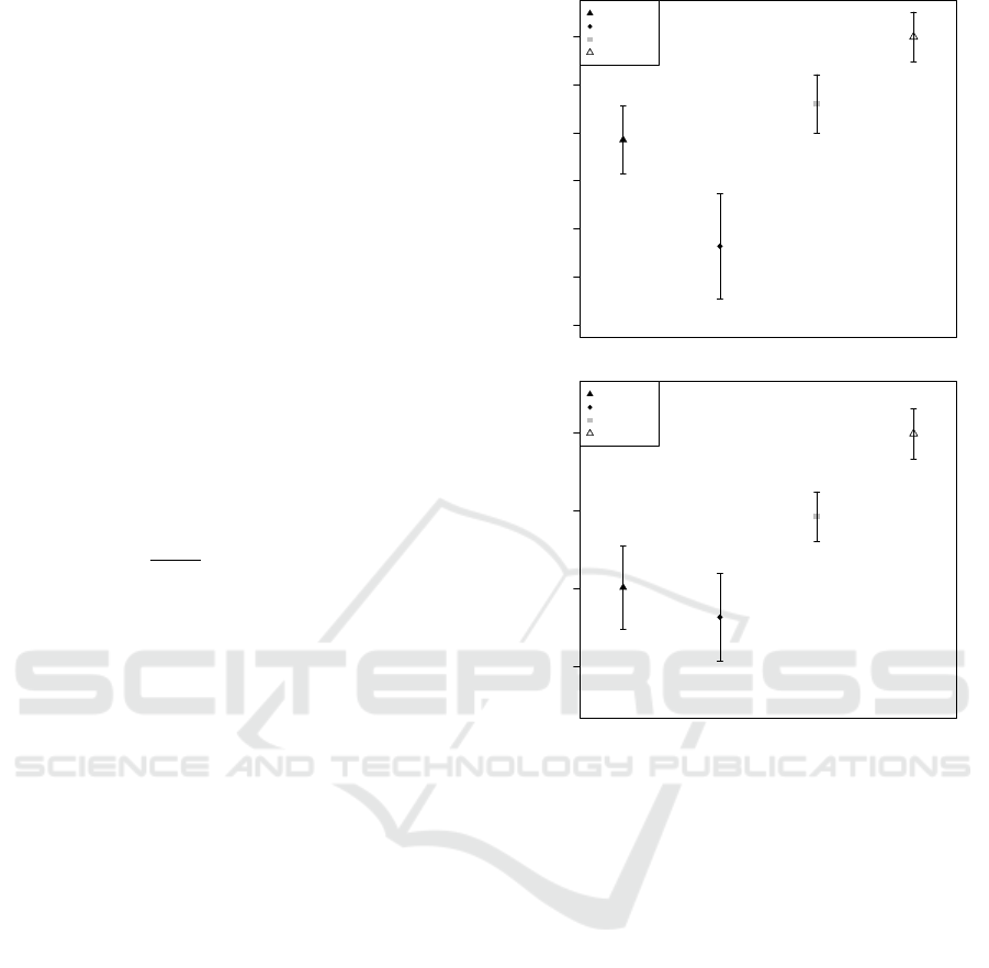
Figure 2: (a) Area under ROC curve and (b) F1-value on NL
dataset.
measurements over 65.537 time steps.(Bodik et al.,
2004)
TURBINE (TU) contains measurements from 39
sensors in a turbine over half an hour with measure-
ments every quarter of a millisecond. This is the
largest of our datasets and contains 39 measurements
over about 8.5 million time steps.(Siemens AG, 2015)
3.3 Experimental Settings
Window size w determines the scale of correlation we
are interested in and eventually has to be chosen by
the user. For the purpose of this evaluation we set it
w = 80 for the synthetic data and equivalent to 1 sec-
ond for the turbine dataset, 30 seconds for the other
sensor datasets, and to 4 weeks for the stock market
dataset. The number of bins b for the discretization
needs to be small enough to avoid singletons in the
histogram but large enough to map the data distribu-
tion – we considered criteria for a sensible choice in
section 2.3. As a compromise we chose b = 20 for
IoTBD 2016 - International Conference on Internet of Things and Big Data
386
0.40 0.45 0.50 0.55 0.60 0.65 0.70
AUC
0.66 0.75 0.85 0.9 0.95 0.99
PeakSim
StatStream
MID
Random
Correlation level
0.x
(a) AUC
0.00 0.05 0.10 0.15 0.20 0.25
F1 max
0.66 0.75 0.85 0.9 0.95 0.99
PeakSim
StatStream
MID
Random
Correlation level
0.x
(b) F1-score
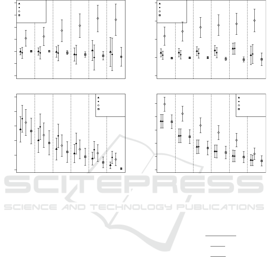
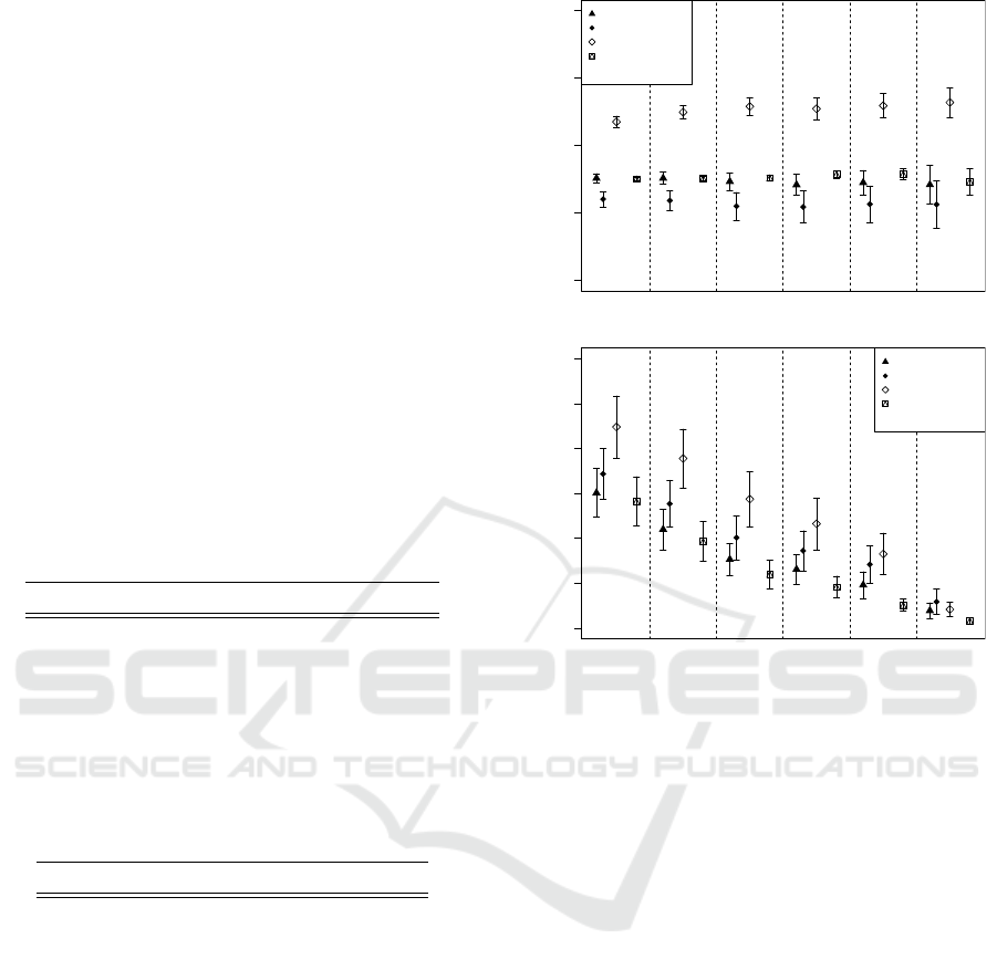
Figure 3: (a) Area under ROC curve and (b) maximum F1-
value on TU dataset. Areas separated by dashed ines show
performance at different levels of desired correlation.
the experiments. PeakSim and StatStream use a pa-
rameter n that determines the number of DFT-peaks
used, and influences runtime and memory in a similar
way b influences MID. Consequently we set n equal
to b, which is very close to the choice of n in (Zhu and
Shasha, 2002) and (Seliniotaki et al., 2014).
We calculate dependency of every dimension with
every other, e.g. voltage with temperature. So, for a
dataset n ×d i.e. with n steps and d dimensions we
calculate (n −w) ·
d
2
dependency scores. Statistical
significance is determined with a standard two-sided
t-test.
3.4 Evaluation Criteria
For the synthetic dataset we provide the area under
ROC curve as classification measure that is indepen-
dent from the number of true positives in the dataset:
AUC = P(X
1
> X
2
), (10)
where X
1
and X 2 are the scores for a positive and neg-
ative instance respectively.
0.4 0.5 0.6 0.7 0.8
AUC
0.66 0.75 0.85 0.9 0.95 0.99
PeakSim
StatStream
MID
Random
Correlation level
0.x
(a) AUC
0.0 0.1 0.2 0.3 0.4 0.5
F1 max
0.66 0.75 0.85 0.9 0.95 0.99
PeakSim
StatStream
MID
Random
Correlation level
0.x
(b) F1-score
Figure 4: (a) Area under ROC curve and (b) maximum F1-
value on OL dataset. Areas separated by dashed lines show
performance at different levels of desired correlation.
Also, we report the F1-measure, i.e. the harmonic
mean of precision and recall:
F1 = 2 ·
precision·recall
precision+recall
, (11)
precision =
T P
T P+FP
, (12)
recall =
T P
T P+FN
. (13)
As a positive in the evaluation we label every instance
as 1 if it is generated from a function, and as 0 if it
is generated by noise (c.f. 3.1). The ground truth to
achieve is then simply the mean of ones and zeros in
a window.
For the datasets where true dependencies are not
known, we chose to evaluate our algorithms at six lev-
els of correlations, from weak to strong correlation,
where we deem a windowed pair of streams with cor-
relation coefficient above 0.66, 0.75, 0.85, 0.9, 0.95
and 0.99 respectively as dependent. Accordingly, we
classify each window as 0 or 1. For each level, we
report for each algorithm AUC and the maximum F1-
score, i.e. the highest F1-score along the precision re-
call curve generated by moving the threshold that sep-
arates predicted positives from predicted negatives.
Detecting Data Stream Dependencies on High Dimensional Data
387
This likely underestimates the number of positives
in the data but provides a lower bound for the perfor-
mance of our algorithm. We see in the synthetic data
how Pearsons’s correlation coefficient underestimates
the dependency of the data streams but performs sur-
prisingly well through linear approximating.
3.5 Results
Figures 2 to 6 show F1-measure (± one standard de-
viation) and AUC (± one standard deviation) for the
five datasets. For the synthetic dataset NL we included
the Pearson’s correlation coefficient. Random has
been determined for the non-synthetic datasets by al-
locating a random value uniformly chosen from [0, 1]
as dependency measure to each pair of stream win-
dows.
Table 1: Direct overview of all (non-synthetic) datasets: We
count significant improvement in AUC (p-value < 0.1 in a
two-sided t-test) of row vs. column in 24 experiments. MID
scores a total of 48.
AUC improvement vs.
MID PkSim SStr
MID - 24 24
PeakSim 0 - 15
StatStream 0 1 -
Table 2: Direct overview of all datasets: We count signifi-
cant improvement in F1 value (p-value < 0.1 in a two-sided
t-test) of row vs. column in 24 experiments. MID scores 33
wins.
F1 improvement vs.
MID PkSim SStr
MID - 19 14
PeakSim 0 - 1
StatStream 5 17 -
Between PeakSim and StatStream we see little
clear difference: PeakSim generally does better than
StatStream in AUC but worse if we look at recall
and precision. Both perform considerably worse than
MID. This holds for both the synthetic and the real
datasets.
In our synthetic data, MID shows close to per-
fect scores, improving significantly (p < 0.1 in a two-
sided t-test) over the correlation- or DFT-based mea-
sures. In the other four datasets it also almost always
improves on the other compared methods.
Considering the area under the ROC curve, we
see our method in the window-based version clearly
outperforming the other correlation measures in all
datasets. Altogether MID significantly outperforms
●
0.2 0.4 0.6 0.8 1.0
AUC
0.66 0.75 0.85 0.9 0.95 0.99
PeakSim
StatStream
MID
Random
Correlation level
0.x
(a) AUC
0.00 0.05 0.10 0.15 0.20 0.25 0.30
F1 max
0.66 0.75 0.85 0.9 0.95 0.99
PeakSim
StatStream
MID
Random
Correlation level
0.x
(b) F1-score
Figure 5: (a) Area under ROC curve and (b) maximum F1-
value on PA dataset. Areas separated by dashed lines show
performance at different levels of desired correlation.
the DFT-based methods in 48 out of 48 direct com-
parisons.
The maximum F1-value shows a similar picture:
We see MID outperforming the DFT-based methods
in 33 out of 48 cases. Table 2 shows the complete ma-
trix of pairwise comparisons for the F1-value. MID
performs well on all data sets, the difference however
tends to fall within the margin of error when higher
levels of correlation are examined where only few
positives are present in the data.
In summary, as proxy for the correlation coeffi-
cient, MID works significantly better than DFT-based
methods based on AUC and F1-score.
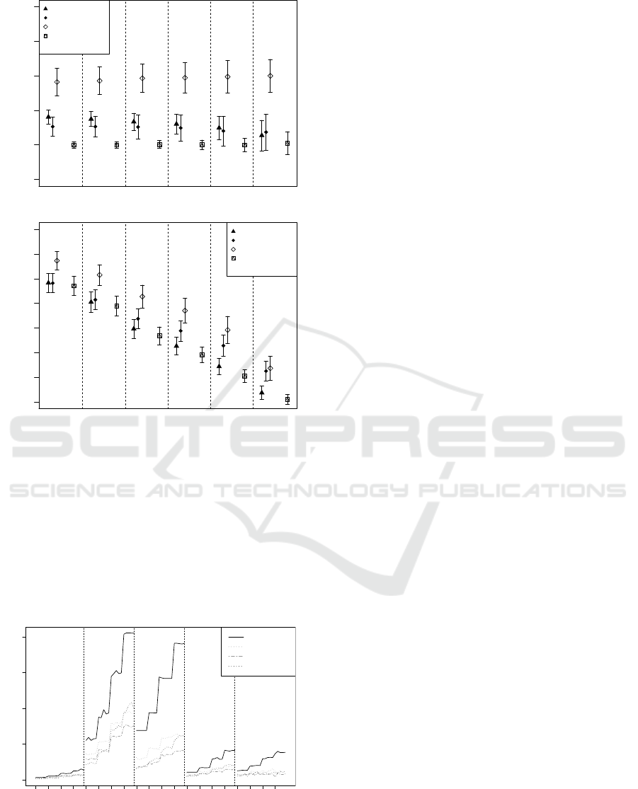
3.6 Execution Time
All experiments have been performed on a PC with an
Intel Xeon 1.80GHz CPU and consumer grade hard-
ware, running a Linux with a current 64-bit kernel,
and implemented in python 3.4. Figure 7 shows exe-
cution times over 5 runs of different correlation mea-
sures.
Considering that the number of pairwise depen-
IoTBD 2016 - International Conference on Internet of Things and Big Data
388
0.4 0.5 0.6 0.7 0.8 0.9
AUC
0.66 0.75 0.85 0.9 0.95 0.99
PeakSim
StatStream
MID
Random
Correlation level
0.x
(a) AUC
0.1 0.2 0.3 0.4 0.5 0.6 0.7 0.8
F1 max
0.66 0.75 0.85 0.9 0.95 0.99
PeakSim
StatStream
MID
Random
Correlation level
0.x
(b) F1-score
Figure 6: (a) Area under ROC curve and (b) maximum F1-
value on NA dataset. Areas separated by dashed lines show
performance at different levels of desired correlation.
dencies grows quadratic in the number of monitored
dimensions, computation speed is an essential factor
to deal with high dimensional data. Clearly, the di-
rect calculation of the correlation coefficient is not
competitive for large datasets and higher data volume
within a window. MID appears about on par with
PeakSim and StatStream.
0 200 400 600 800
window length
time/s
20 40 80 120 20 40 80 120 20 40 80 120 20 40 80 120 20 40 80 120
CorrCoeff
PeakSim
StatStream
MID
Figure 7: Execution time averaged over 5 runs with increas-
ing window length on the (from left to right) NL, TU, OL,
PA and NA dataset.
4 CONCLUSION
We developed mutual information, a concept from in-
formation theory, into a metric that can help to eval-
uate sensor readings or other streaming data. We de-
scribe an incremental algorithm to compute our mu-
tual information based measure with time complexity
linear to the length of the data streams. The compet-
itive execution time is achieved with a suitable dis-
cretization technique. We evaluated our algorithm on
four real life datasets with up to 8.5 million records
and against two other algorithms to detect correlations
in data streams. It is as more accurate for detecting
dependencies in the data than other approximation al-
gorithms.
In future work we want to address the choice of
a suitable parameter value for the window length or
eliminate the static window altogether. Extending the
search for dependencies from pairwise to groups of
3 or more streams increases the computational com-
plexity but brings the potential to extend the analysis
to an entropy-based ad-hoc clustering.
Mutual information brings a different perspective
to stream analysis that is independent from assump-
tions on the distribution of or relationship between the
data streams.
REFERENCES
Bernhard, H.-P., Darbellay, G., et al. (1999). Performance
analysis of the mutual information function for non-
linear and linear signal processing. In Acoustics,
Speech, and Signal Processing, 1999. Proceedings.,
1999 IEEE International Conference on, volume 3,
pages 1297–1300. IEEE.
Bodik, P., Hong, W., Guestrin, C., Madden, S., Paskin,
M., and Thibaux, R. (2004). Intel lab data.
http://db.csail.mit.edu/labdata/labdata.html.
Cover, T. M. (1991). Ja thomas elements of information
theory.
Darbellay, G. A. (1999). An estimator of the mutual in-
formation based on a criterion for conditional inde-
pendence. Computational Statistics & Data Analysis,
32(1):1–17.
Daub, C. O., Steuer, R., Selbig, J., and Kloska, S.
(2004). Estimating mutual information using b-
spline functions–an improved similarity measure for
analysing gene expression data. BMC bioinformatics,
5(1):118.
Dionisio, A., Menezes, R., and Mendes, D. A. (2004). Mu-
tual information: a measure of dependency for nonlin-
ear time series. Physica A: Statistical Mechanics and
its Applications, 344(1):326–329.
Fernandez, D. A., Grau-Carles, P., and Mangas, L. E.
(2002). Nonlinearities in the exchange rates returns
Detecting Data Stream Dependencies on High Dimensional Data
389

and volatility. Physica A: Statistical Mechanics and
its Applications, 316(1):469–482.
Friedman, J. H. (2001). Greedy function approximation: a
gradient boosting machine. Annals of statistics, pages
1189–1232.
Granger, C. and Lin, J.-L. (1994). Using the mutual infor-
mation coefficient to identify lags in nonlinear mod-
els. Journal of time series analysis, 15(4):371–384.
Hall, P. and Morton, S. C. (1993). On the estimation of
entropy. Annals of the Institute of Statistical Mathe-
matics, 45(1):69–88.
Han, M., Ren, W., and Liu, X. (2015). Joint mutual
information-based input variable selection for multi-
variate time series modeling. Engineering Applica-
tions of Artificial Intelligence, 37:250–257.
Kalu
ˇ
za, B., Mirchevska, V., Dovgan, E., Lu
ˇ
strek, M., and
Gams, M. (2010). An agent-based approach to care
in independent living. In Ambient intelligence, pages
177–186. Springer.
Kraskov, A., St
¨
ogbauer, H., and Grassberger, P. (2008).
Estimating mutual information. Physical review E,
69(6):066138.
Paninski, L. (2003). Estimation of entropy and mutual in-
formation. Neural computation, 15(6):1191–1253.
Seliniotaki, A., Tzagkarakis, G., Christofides, V., and
Tsakalides, P. (2014). Stream correlation monitor-
ing for uncertainty-aware data processing systems.
In Information, Intelligence, Systems and Applica-
tions, IISA 2014, The 5th International Conference on,
pages 342–347. IEEE.
Siemens AG (2015). Gas turbine data. .
Sorjamaa, A., Hao, J., and Lendasse, A. (2005). Mutual in-
formation and k-nearest neighbors approximator for
time series prediction. Artificial Neural Networks:
Formal Models and Their Applications–ICANN 2005,
pages 752–752.
The NASDAQ Stock Market (2015). Nasdaq daily quotes.
http://www.nasdaq.com/quotes/nasdaq.
Zhu, Y. and Shasha, D. (2002). Statstream: Statistical mon-
itoring of thousands of data streams in real time. In
Proceedings of the 28th international conference on
Very Large Data Bases, pages 358–369. VLDB En-
dowment.
IoTBD 2016 - International Conference on Internet of Things and Big Data
390
