
The Growth of Oligarchy in a Yard-Sale Model of Asset Exchange
A Logistic Equation for Wealth Condensation
Bruce M. Boghosian, Adrian Devitt-Lee and Hongyan Wang
Department of Mathematics, Tufts University, Medford, Massachusetts, U.S.A.
Keywords:
Fokker-Planck Equation, Asset Exchange Model, Yard-Sale Model, Pareto Distribution, Gibrat’s Law,
Lorenz Curve, Gini Coefficient, Lorenz-Pareto Exponent, Phase Transitions, Phase Coexistence, Wealth
Condensation.
Abstract:
The addition of wealth-attained advantage (WAA) to the Yard-Sale Model (YSM) of asset exchange has been
demonstrated to induce wealth condensation. In models of WAA for which the bias is a continuous function
of the wealth difference of the transacting agents, the condensation arises from a second-order phase transition
to a coexistence regime. In this paper, we present the first analytic time-dependent results for this model, by
showing that the condensed wealth obeys a simple logistic equation in time.
1 INTRODUCTION
The scientific study of wealth inequality is motivated
by a desire to understand not only the drastic uneven-
ness in the distribution of wealth today, but also its dy-
namism. Virtually every metric of wealth inequality
is changing in the direction of increased concentration
of wealth. For example, in 2010 Oxfam International
noted that 388 individuals in the world had as much
wealth as half the human population. They have been
publishing this figure annually, and by early 2016 it
had reduced to 62 individuals (Hardoon and Ayele,
2016).
An important class of wealth distribution models
that have been analyzed using mathematical methods
of statistical physics are called Asset Exchange Mod-
els (AEMs) (Angle, 1986; Hayes, 2002). These have
been used to describe the collective behavior of large
economic systems based on simple, idealized micro-
scopic rules. In a simple AEM, there exists a col-
lection of N agents, each of whom possesses some
wealth. The agents exchange that wealth in pairwise
transactions. There are a variety of models describing
these transactions. Most conserve the total number
of agents, N, and the total wealth in the system, W,
though extended versions of these models are capa-
ble of accounting for wealth redistribution, changes
in agent population, the production and consumption
of wealth, and multi-agent transactions.
The AEM examined in this paper is a modifica-
tion of the basic Yard Sale Model (YSM) of asset ex-
change (Chakraborti, 2002; Hayes, 2002), in which
agents exchange wealth solely by means of pairwise
transactions. When two agents enter such a transac-
tion, each has the same probability of winning some
amount of wealth from the other, and the amount won
is equal to a fraction of the poorer agent’s wealth.
Following the work of Ispolatov et al. (Ispolatov
et al., 1998), Boghosian derived a Boltzmann equa-
tion for the basic YSM (Boghosian, 2014b). In the
limit of small transactions, he showed that the Boltz-
mann equation reduces to a particular Fokker-Planck
(FP) equation, and later demonstrated that this FP
equation could be derived much more simply from
a stochastic process (Boghosian, 2014a). In the ab-
sence of any kind of wealth redistribution, Boghosian
et al. (Boghosian et al., 2015) proved that all of the
wealth in the system is eventually held by a single
agent. This is due to a subtle but inexorable bias in
favor of the wealthy in the rules of the YSM: Be-
cause a fraction of the poorer agent’s wealth is traded,
the wealthy do not stake as large a fraction of their
wealth in any given transaction, and therefore can
lose more frequently without risking their status. This
is ultimately due to the multiplicative nature of the
transactions on the agents’ wealth, as pointed out by
Moukarzel (Moukarzel et al., 2007).
In the above-mentioned works, Boghosian et
al. (Boghosian, 2014b; Boghosian, 2014a; Boghosian
et al., 2015) also investigated the addition of a sim-
ple Ornstein-Uhlenbeck-like model of redistribution
to the YSM (Uhlenbeck and Ornstein, 1930). They
Boghosian, B., Devitt-Lee, A. and Wang, H.
The Growth of Oligarchy in a Yard-Sale Model of Asset Exchange - A Logistic Equation for Wealth Condensation.
In Proceedings of the 1st International Conference on Complex Information Systems (COMPLEXIS 2016), pages 187-193
ISBN: 978-989-758-181-6
Copyright
c
2016 by SCITEPRESS – Science and Technology Publications, Lda. All rights reserved
187

demonstrated that it suppressed the tendency of all
the wealth to go to a single agent, resulting in a
classical distribution, and exhibiting some similar-
ity with empirical forms for wealth distributions due
to Pareto (Pareto, 1965) and Gibrat (Gibrat, 1931).
In later work, however, they demonstrated that the
extreme tail of this distribution decays as a gaus-
sian (Boghosian et al., 2016).
The phenomenon of wealth condensation was
first described by Bouchard and M´ezard in 2000,
who noted the accumulation of macroscopic levels of
weath by a single agent in a simple model of trading
and redistribution (Bouchaud and M´ezard, 2000). In
2007, Moukarzel et al. investigated wealth-attained
advantage (WAA) in the YSM by adding a fixed bias
to the probability of winning in any transaction, de-
pendent only on the sign of the wealth differential.
He observed a first-order phase transition to a wealth-
condensed state of absolute oligarchy, in which a sin-
gle agent held all the wealth (Moukarzel et al., 2007).
More recently, Boghosian et al. (Boghosian et al.,
2016) introduced a new model for WAA in the YSM,
with bias favoring the wealthier agent proportional to
the wealth differential between the two agents, thus
approaching zero continuously for transactions be-
tween agents of equal wealth. This model exhibits a
second-order phase transition to a state of coexistence
between an oligarch and a classical distribution of
non-oligarchs. In that work it was also demonstrated
that the above-mentioned gaussian tail was present
both below and above criticality, but degenerated to
exponential decay precisely at criticality.
While it is perhaps unsurprising that WAA pro-
motes the condensation of wealth, the above obser-
vation demonstrates that the way it is introduced
can have macroscopic consequences. In a first-order
phase transition, order parameters, such as the Gini
coefficient or the fraction of wealth held by the
wealthiest agent in this case, are discontinuous func-
tions of the control parameters. In a second-order
phase transition, they exhibit only slope discontinu-
ities. It seems, therefore, that the continuity or dis-
continuity of the bias in the microscopic model is di-
rectly reflected in the continuity or discontinuity of
the macroscopic order parameter.
To be specific, if the coefficient τ
∞
measures the
level of redistribution for the wealthiest agents, and ζ
measures the level of WAA (in a fashion made pre-
cise in (Boghosian et al., 2016)), then criticality was
shown to occur at ζ = τ
∞
, and coexistence for ζ > τ
∞
.
The fraction of wealth held by the oligarch in the con-
tinuum limit was shown to be
c
∞
=
0 if ζ ≤ τ
∞
1−
τ
∞
ζ
if ζ > τ
∞
(1)
Note that this is a continuous function, with a discon-
tinuous first derivative at the critical point ζ = τ
∞
, re-
flective of a second-order phase transition.
Note that all of the above-described observations
were made for the steady state situation. In this pa-
per we quantify the time dependence of the formation
of partial oligarchy in the model (Boghosian et al.,
2016). We derive a PDE, valid in the coexistence
regime ζ > τ
∞
, governing the distribution of wealth
p(w,t) amongst the non-oligarchs, coupled with an
ODE for the fraction of wealth held by the oligarch,
c(t). The latter is the logistic equation
c
′
(t) = c(t)[−τ
∞
+ ζ(1−c(t))], (2)
whose long-time limit c
∞
:= lim
t→∞
c(t) is consistent
with Eq. (1) for ζ > τ
∞
.
In Section 2 we describe the YSM, and the deriva-
tion of the FP equation describing its behavior. In
particular, we review the assumptions and methodol-
ogy of the Kramers-Moyal derivation of the FP equa-
tion from a stochastic process, because these assump-
tions are violated by the singular distributional solu-
tions that we shall be studying.
In Section 3 we provide a mathematical descrip-
tion for oligarchy as the presence of a singular dis-
tribution Ξ, correct the Kramers-Moyal derivation of
the FP equation, and present the logistic ODE that de-
scribes the wealth of the oligarch. For reasons dis-
cussed in the conclusions, this decouples from the
PDE governing the distribution of non-oligarchs.
2 THE YARD SALE MODEL
In this section we will introduce notation, discuss
the interaction between agents in the modified YSM,
and review the assumptions and methodology of the
Kramers-Moyal derivation of the FP equation from a
stochastic process. While this section follows that of
(Boghosian et al., 2016) closely, this review is neces-
sary because we shall require a weak form of the FP
equation in order to accommodate distributional solu-
tions in what follows.
A continuous distribution of wealth can be de-
scribed by the agent density function (ADF), P(w,t),
defined such that the number of agents with wealth
w ∈ [a,b] at time t is given by
R
b
a
P(w,t)dw. The ze-
roth and first moments of the ADF correspond to the
total number of agents and wealth,
N
P
:=
Z
∞
0
dw P(w,t),
W
P
:=
Z
∞
0
dw P(w,t)w.
COMPLEXIS 2016 - 1st International Conference on Complex Information Systems
188

We will often need the three following partial mo-
ments:
A
P
(w,t) :=
Z
∞
w
dx
P(x,t)
N
P
,
L
P
(w,t) :=
Z
w
0
dx
P(x,t)
N
P
x,
B
P
(w,t) :=
Z
w
0
dx
P(x,t)
N
P
x
2
2
.
Here A
P
(w) denotes the Pareto potential, which is the
fraction of agents with wealth at least w. Also, L
P
(w)
is the Lorenz potential, which denotes the fraction of
wealth held by agents with wealth up to w. In the fol-
lowing sections, the expectation of functions over the
ADF will be denoted as E
x
[ f (x)] :=
R
∞
0
dx
P(x,t)
N
P
f(x).
To describe the dynamics of wealth distributions,
we use a random walk based on the YSM, in which
two agents are randomly chosen to transact, and the
magnitude of wealth exchanged is a fraction of the
minimum wealth of the two agents. The winner is
determined by a random variable η ∈ {−1, +1}. If
we focus on a single agent whose wealth transitions
from z to w as a result of the transaction, this gives
rise to the random walk
w−z = η
√
∆tmin(z,x),
where
√
∆t is a measure of the transactional timescale
and x is the wealth of the “other agent” with whom the
agent in question interacts.
We now introduce redistribution: After each trans-
action, a wealth tax is imposed on each agent, and
the total amount collected is redistributed amongst all
the agents in the system. The fraction collected from
an agent with wealth z per unit time is denoted by
τ(z), so the total tax collected per unit time is T
P
(t) =
R
∞
0
dz P(z,t)τ(z)z. The average amount returned to
each agent per unit time is T
P
/N
P
, and the fractional
deviation from this average amount for an agent of
wealth z will be denoted by σ(z), so the amount re-
turned to that agent is T
P
/N
P
+ σ(z)z. Hence the net
taxation experienced by an agent with wealth z is
τ(z)z−
T
P
N
P
+ σ(z)z
= ρ(z)z−
T
P
N
P
,
where we have defined ρ(z) := τ(z) −σ(z). Note
that lim
z→∞
σ(z) = 0, so τ
∞
:= lim
z→∞
τ(z) =
lim
z→∞
ρ(z) =: ρ
∞
. Because the total amount col-
lected must be equal to the total amount redistributed,
the expectation value of the deviation from average
redistribution must vanish, whence 0 = E
z
[σ(z)z] and
T
P
(t) =
Z
∞
0
dz P(z,t)ρ(z)z. (3)
For example, if we assume that τ(z) is a constant,
independent of z, we find that
T
P
(t) =
Z
∞
0
dz P(z)τz = τW
P
is also constant. If we further take σ(z) = 0, so that
the redistribution is uniform, we see that the total ef-
fective taxation rate is
τz−
T
P
N
P
= τz−
τW
P
N
P
= τ
z−
W
P
N
P
.
This redistribution model is reminiscent of the
Ornstein-Uhlenbeck process (Uhlenbeck and Orn-
stein, 1930), and has been used in recent studies of
the redistributive YSM (Boghosian et al., 2016).
The addition of redistribution determines a new
random walk for an individual agent, defined by
w−z = −
ρ(z)z−
T
P
N
P
∆t + η
√
∆tmin(z,x). (4)
We see that only the difference ρ(z) := τ(z) −σ(z)
matters, in terms of which T
P
(t) is given by Eq. (3). In
what follows, we shall allow for ρ to be negative, but
we will require that it be bounded by a polynomial.
The random variable η can be distributed fairly
(with mean E[η] = 0), or it can be biased. The bias
assumed in this paper is that for a model of WAA de-
scribed in an earlier paper (Boghosian et al., 2016),
specifically
E [η] = ζ
N
P
W
P
√
∆t(z−x), (5)
where ζ is a positive parameter that skews the proba-
bility of winning in favor of the wealthier agent. Thus,
in this model, the bias is determined by the difference
between the wealth of the two agents.
We will work from Eq. (4) from the start, and
simpler systems can be obtained by letting ζ = 0 or
τ(w) = 0. We shall first formally derive a PDE which
is implied by the random walk in the limit as the frac-
tion of wealth traded becomes infinitesimal.
We suppose that the probability of the transition
(z,t) → (w,t + ∆t) is p
∆t
(z → w;z,t), and that this
probability distribution is normalized. The Chapman-
Kolmogorov equation for this random walk is then
P(w,t + ∆t) =
Z
∞
0
dz P(z,t)p
∆t
(z → w;z,t)
To derive the corresponding FP equation satisfied by
P, we must cast the above in weak form. To this end,
we let ψ be an analytic Schwartz function on the do-
main [0,∞), and compute its L
2
inner product with
The Growth of Oligarchy in a Yard-Sale Model of Asset Exchange - A Logistic Equation for Wealth Condensation
189

∂P/∂t as follows,
ψ,
∂P
∂t
=
Z
ψ(w)
∂P(w,t)
∂t
= lim
∆t→0
1
∆t
Z
dwψ(w)P(w,t + ∆t) −
Z
dwψ(w)P(w,t)
= lim
∆t→0
1
∆t
Z
dzP(z,t)
Z
dw p
∆t
(z →w;z,t)[ψ(w) −ψ(z)]
= lim
∆t→0
1
∆t
Z
dzP(z,t)
Z
dw p
∆t
(z →w;z,t)
∞
∑
n=1
(w−z)
n
n!
∂
n
ψ(z)
∂z
n
=
∞
∑
n=1
1
n!
Z
dzM
n
(z,t)P(z,t)
∂
n
ψ(z)
∂z
n
(6)
where we have defined
M
n
(z,t) := lim
∆t→0
1
∆t
Z
dw p
∆t
(z → w;z,t)(w−z)
n
= E
x,η
(w−z)
n
∆t
.
The above result may be written
ψ,
∂P
∂t
=
∞
∑
n=1
1
n!
M
n
(z,t)P(z,t),
∂
n
ψ(z)
∂z
n
. (7)
whence, using integration by parts to revert to the
strong form, we obtain
∂P
∂t
=
∞
∑
n=1
(−1)
n
n!
∂
n
z
[M
n
(z,t)P(z,t)] , (8)
and thus the agent density function satisfies a PDE
that is determined by the moments of the random walk
on an infinitesimal timescale.
2.1 Fokker-Planck equation
Recalling Eqs. (4) and (5), we can compute M
1
,
M
1
(z,t)
= lim
t→0
E
η,x
(w−z)
∆t
= E
x
T
P
(t)
N
P
−zρ(z) + ζ
N
P
W
P
(z−x)min(w,x)
=
T
P
(t)
N
P
−zρ(z) −ζ
2
N
P
W
P
B
P
(z,t) −2zL
P
(z,t) −z
2
N
P
W
P
A
P
(z,t) + z
(9)
Next, because η ∈ {−1, +1}, we have E
η
[η
2
] = 1,
which allows us to compute M
2
,
M
2
(z,t)
= lim
t→0
E
η,x
(w−z)
2
∆t
= lim
t→0
E
η,x
∆t(
T
P
(t)
N
P
−zρ(z))
2
+(
T
P
(t)
N
P
−zρ(z))ηmin(z,x)(∆t)
1/2
+ η
2
min(z,x)
2
= E
η,x
η
2
min(z, x)
2
=
Z
∞
0
dx
P(x,t)
N
P
min(z, x)
2
= 2B
P
(z,t) + z
2
A
P
(z,t). (10)
Finally, we note that higher powers of η have expec-
tations E
η
[η
k
] ≤ 1 for k ≥ 3. It follows that, because
each term in the expansion of the above equation in-
cludes some positive power of
√
∆t, all of the mo-
ments approach zero for k ≥ 3,
M
k
(z,t) = lim
t→0
1
∆t
E
η,x
"
∆t[
T
P
(t)
N
P
−zρ(z)] + η
√
∆tmin(w,x)
k
#
= 0.
(11)
Substituting Eqs. (9), (10) and (11) into Eq. (8),
we find that our wealth distribution obeys the fol-
lowing quadratically nonlinear, integrodifferential FP
equation,
∂P
∂t
+
∂
∂w
T
P
(t)
N
P
−wρ(w)
P
=
∂
2
∂w
2
B
P
+
w
2
2
A
P
P
+
∂
∂w
ζ
N
P
W
P
2B
P
−2wL
P
−w
2
N
P
W
P
A
P
+ w
P
.
(12)
This system conserves wealth and agents, as was
shown in the appendix of the paper where it was first
derived (Boghosian et al., 2016). In the case where
there is no redistribution and no WAA, we have τ =
ζ = 0, so the agent density function satisfies
∂P
∂t
=
∂
2
∂w
2
B
P
(w,t) +
w
2
2
A
P
(w,t)
P
. (13)
2.2 Oligarchy as a Distributional
Solution
The steady-state solution to Eq. (12) may involve
the condensation of a finite fraction of the system’s
wealth into the hands of a vanishingly small number
of agents. Indeed, in the absence of redistribution, as
in Eq. (13), all the wealth will condense in this man-
ner. To describe this, we must extend our function
space to include certain singular distributions.
If our system were discrete, then complete con-
centration of wealth would be described by P(w) =
(N
P
−1)δ(w)+δ(w−W
P
), where N
P
−1 agents have
no wealth, and a single agent holds all of the wealth.
In the continuum limit, however, the number of agents
need not be an integer. Thus wealth condensation
could continue indefinitely, with a “half an agent”
holding twice the wealth of the system, described
by the distribution P(w) = (N
P
−
1
/2)δ(w) +
1
/2δ(w−
2W
P
). More generally, we can take the distribution to
be P(w) = (N
P
−ε)δ(w) + εδ(w−W
P
/ε), where ε is
an arbitrarily small positive number. Replacing ε by
W
P
ε and passing to the limit as ε → 0 yields
P(w) = N
P
δ(w) +W
P
Ξ(w), (14)
COMPLEXIS 2016 - 1st International Conference on Complex Information Systems
190

where we have defined Ξ(w) = lim
ε→0
εδ(w −1/ε).
To be more precise, Ξ should be defined as the singu-
lar distribution whose action on a test function φ is
hΞ,φi= lim
ε→0
ε
δ
w−
1
ε
,φ
= lim
ε→0
ε φ
1
ε
= lim
s→∞
φ(s)
s
. (15)
Here the space of test functions to which φ belongs is
∂
−2
S
0
= {φ(w) = ψ(w) + γ+ µw : ψ(w) ∈ S ([0,∞)),γ,µ ∈R},
where S([0,∞) denotes Schwartz functions on [0,∞).
3 WAA ABOVE CRITICALITY
In this section, we use the definition of Ξ provided
by Eq. (15). In earlier work (Boghosian et al., 2016),
the FP equation, Eq. (12), and its steady-state asymp-
totic behavior were discussed in detail. A second-
order phase transition was observed at the critical
point ζ = τ
∞
, and coexistence was observed between
the singular distribution Ξ and a classical distribution
for ζ > τ
∞
. This may be thought of as an oligarch in
coexistence with a population of non-oligarchs. The
presence of the singular distribution Ξ, however, vio-
lates the assumptions in the derivation of the FP equa-
tion, as our presentation leading to Eq. (8) assumed an
analytic Schwartz function in the weak form.
Recall that the mathematical phenomenon that we
describe here as “oligarch” may be modeled as the
wealth held by the wealthiest fraction ε of agents,
as ε → 0. Assume that there exists a wealth dis-
tribution which is a steady state of the random pro-
cess, Eq. (4), in the small-transaction limit. More-
over, suppose that this distribution may be written as
P(w) = p(w)+ c(t)W
P
Ξ(w), where p(w) is the classi-
cal agent density function for the non-oligarchs. This
is a system in which the wealthiest infinitesimal of
agents hold a fraction c(t) of the total wealth of the
system at time t. We consider two sets of agents in
the random walk: There are the “normal” agents, cor-
responding to the classical distribution p(w). Then
there is what we have been calling the “oligarch,” con-
sidered to be the wealthiest fraction ε of the distribu-
tion P(w), considered as a single unit.
Now suppose that we have an oligarch, and φ =
ψ+ γ+ µw, where ψ is an analytic Schwartz function.
Then the development that led to Eq. (6) becomes:
∂P
∂t
,φ
=
∞
∑
n=1
1
n!
Z
M
n
(z,t)P(z,t)
∂
n
φ(z)
∂z
n
dz
=
∞
∑
n=1
1
n!
Z
[M
n
(z,t)P(z,t)]∂
n
z
ψ+ µM
1
(z,t)P(z,t)dz
=
∞
∑
n=1
1
n!
Z
∂
n
z
[M
n
(z,t)P(z,t)]ψdz
!
+ µN
P
E
z
[M
1
(z,t)]. (16)
In strong form we therefore have
∂P
∂t
=
∞
∑
n=1
(−1)
n
n!
∂
n
z
[M
n
(z,t)P(z,t)]
!
+ E
z
[M
1
(z,t)]N
P
Ξ,
where the Ξ term arises from hM
1
(z,t)P(z,t),µi =
µhP(z,t),M
1
(z,t)i = hΞ,φi·N
P
E
z
[M
1
(z,t)]. This im-
plies two things: the strong form of the FP equation
may not make sense in the coexistence regime, and Ξ
is likely to depend only on the M
1
term, which corre-
sponds to drift in the FP equation.
To carry out the full analysis, we must recalcu-
late the coefficients M
n
(z,t) for three cases: (i) a nor-
mal agent interacting with another normal agent, (ii)
a normal agent interacting with the oligarch, and (iii)
the oligarch interacting with a normal agent. The
first two factors would describe p(w,t), and the last
would determine c(t), the fraction of wealth held by
the oligarch. In this paper, we restrict our attention to
the wealth of the oligarch only, and we relegate the
derivation of the PDE governing the non-oligarchical
portion of the distribution to future work.
Denote the first coefficient M
1
of the wealthiest ε
of agents by M
ε
1
. Instead of using the full machinery
of the FP derivation, we note
M
ε
1
(z,t) = lim
t→0
E
η,x
c(t + ∆t)W
P
/ε−c(t)W
P
/ε
∆t
= c
′
(t)
W
P
ε
= T
P
(t) −c(t)
W
P
ε
τ
c(t)W
P
ε
+ E
x
ζ
N
P
W
P
c(t)W
P
ε
−x
x
= T
P
(t) −(c(t)W
P
/ε)τ(c(t)W
P
/ε)
+ ζ
1
W
P
[c(t)W
2
P
(1−c(t))/ε −2N
P
B
p
(c(t)W
P
/ε)],
where the integrals for the expectation are between
x = 0 and x = cW
P
/ε, so that they do not include
the oligarch. We will assume that p decays like an
exponential or a gaussian, as was shown in earlier
work (Boghosian et al., 2016). Under this assump-
tion, the second moment of p is finite, so when we
take the limit as ε → 0, we have
c
′
(t) = c(t)[−τ
∞
+ ζ(1−c(t))], (17)
where we have written τ
∞
:= lim
ε→0
τ(1/ε). This is a
logistic equation for c(t) with solution
c(t) = (1−τ
∞
/ζ)
c
0
e
(ζ−τ
∞
)t
c
0
(e
(ζ−τ
∞
)t
−1) + 1−τ
∞
/ζ
. (18)
Eq. (17) is the principal result of this paper. It indi-
cates that the wealth of the oligarch obeys a logistic
The Growth of Oligarchy in a Yard-Sale Model of Asset Exchange - A Logistic Equation for Wealth Condensation
191
equation, independent of the evolution of the classical
portion of the wealth distribution.
Equation (17) indicates that there are two asymp-
totic solutions in time, one at c= 0, and another at c=
1−τ
∞
/ζ. Since
d
dc
[c((1−c)ζ−τ
∞
)]
c=0
= (ζ −τ
∞
),
the absence of an oligarch is stable if ζ < τ
∞
, and
is unstable otherwise. Similarly, the presence of an
oligarch is stable if ζ > τ
∞
, and is unstable other-
wise
1
Furthermore, since the presence of an oligarch
implies that there is finite taxation on the wealthi-
est agent, τ
∞
must exist. Monte Carlo simulations
confirm the stable steady state of the oligarch both
above and below criticality: The wealth held by the
wealthiest agent, plotted in Fig. 1, is of the same or-
der as that of all the other agents, and is approximately
c = 1−τ
∞
/ζ above criticality.
Figure 1: Monte Carlo simulation of the wealth held by the
wealthiest agent in simulations of different sizes, with var-
ious values of constant τ and σ. As the number of agents
grows, this approaches the theoretical result c = 1−τ
∞
/ζ.
3.1 Gini coefficients above criticality
Finally, we wish to define the notion of Gini coeffi-
cient in the coexistence region above criticality. In
particular, we wish to describe the Gini coefficient of
the entire system in terms of that of the classical sys-
tem p, excluding the oligarch. The phenomenon of
oligarchy is evidenced by a Lorenz curve that does
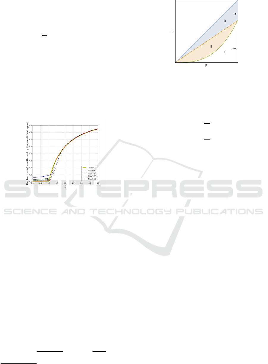
not reach the point (1,1), as illustrated in Fig. 2, where
we have labelled three distinct regions below the di-
agonal. We shall use the labels “I”, “II” and “III” to
denote the areas of these regions. Since the fraction
c of the wealth of the system is held by the infinitesi-
mal agent described by the oligarch, the Lorenz curve
will reach the point (1,1-c). So if we consider the Gini
coefficient of the system p, then we know that:
G
P
=
II + III
I + II + III
, G
p
=
II
I + II
(19)
1
Note that we never have a stable oligarch with negative
wealth; if c = 1−τ
∞
/ζ < 0, then ζ < τ
∞
.
Figure 2: Lorenz plot with partial wealth condensation. A
fraction c of the wealth has condensed, and 1 − c is dis-
tributed classically.
Clearly I + II + III = 1/2, I + II = (1 −c)/2, and
III = c/2. Using the supercritical value of c, this im-
mediately implies that
G
P
= +1+
τ
∞
ζ
(1−G
p
) (20)
G
p
= −1+
ζ
τ
∞
(1−G
P
). (21)
These equations are straightforward relations between
the versions of the Gini coefficient defined with and
without the presence of the oligarch.
4 DISCUSSION AND
CONCLUSIONS
Coexistence between wealth-condensed and normal
distributions in steady-state solutions of the YSM was
first noted in earlier work (Boghosian et al., 2016).
This paper provides the first exact analytic result for
the time-dependent behavior of that model. In partic-
ular, it demonstrates that the fraction of wealth held
by the oligarch above criticality obeys a logistic equa-
tion, Eq. (17). This equation is remarkable in that it
is completely decoupled from the classical part of the
distribution, p(w), and may be solved exactly.
The reason that the equation for c(t) decouples
from that for the classical part of the distribution can
be understood by noting that the oligarch always wins
in transactional exchanges with non-oligarchs. From
the point of view of the oligarch, the remainder of the
distribution might as well be aggregated into a sin-
gle agent with wealth W
p
= (1 −c)W
P
who, oblig-
ingly, always loses in any transaction with the oli-
garch. The oligarch’s ability to gain wealth from the
non-oligarchical portion of the distribution is there-
fore limited only by the rate at which he/she transacts
with non-oligarchs, as compared to the rate at which
he/she is taxed. This is why the steady-state fraction
of wealth held by the oligarch depends only on the
ratio of tax rate to WAA rate, τ
∞
/ζ.
COMPLEXIS 2016 - 1st International Conference on Complex Information Systems
192

From a macroeconomic perspective, it is well
known that most real-world oligarchs worry much
less than the rest of the population about individual
transactions; beyond a certain point, many do not even
know where their own money is invested. By con-
trast, they worry deeply about how taxation and re-
distribution affect their fortunes, and they expend sig-
nificant effort to lobby against progressive taxation,
capital gains taxes and inheritance taxes. We believe
that the asymptotic analysis of the YSM may provide
a way to understand these priorities.
REFERENCES
Angle, J. (1986). The surplus theory of social stratification
and the size distribution of personal wealth. Social
Forces, 65:293–326.
Boghosian, B. (2014a). Fokker-planck description of
wealth dynamics and the origin of pareto’s law. Inter-
national Journal of Modern Physics C, 25:1441008–
1441015.
Boghosian, B. (2014b). Kinetics of wealth and the pareto
law. Physical Review E, 89:042804–042825.
Boghosian, B., Devitt-Lee, A., Johnson, M., Marcq, J., and
Wang, H. (2016). Oligarchy as a phase transition:
The effect of wealth-attained advantage in a fokker-
planck description of asset exchange. arXiv preprint
arXiv:1511.00770v2 [physics.soc-ph]
.
Boghosian, B., Johnson, M., and Marcq, J. (2015). An
h theorem for boltzmann’s equation for the yard-
sale model of asset exchange. Journal of Statistical
Physics, 161:1339–1350.
Bouchaud, J.-P. and M´ezard, M. (2000). Wealth conden-
sation in a simple model of the economy. Physica A,
282:536–545.
Chakraborti, A. (2002). Distributions of money in model
markets of economy. Int. J. Mod. Phys. C, 13:1315–
1321.
Gibrat, R. (1931). Les In´egalit´es ´economiques. Paris: Sirey.
Hardoon, D. and Ayele, S. (2016). An economy for the
1%. Technical report, Oxfam International. 210 Ox-
fam Briefing Paper (Oxfam Davos Report).
Hayes, B. (2002). Follow the money. American Scientist,
90:400–405.
Ispolatov, S., Krapivsky, P., and Redner, S. (1998). Wealth
distributions in asset exchange models. The European
Physical Journal B – Condensed Matter, 2:267–276.
Moukarzel, C., Gonc¸alves, S., Iglesias, J., and Huerta-
Quintanilla, R. (2007). Wealth condensation in a mul-
tiplicative random asset exchange model. Europhys.
J. Spec. Topics, 143:75–79.
Pareto, V. (1965). La courbe de la repartition de la richesse.
In Busino, G., editor, Oevres Completes de Vilfredo
Pareto, page 15. Geneva: Librairie Droz.
Uhlenbeck, G. and Ornstein, L. (1930). On the theory of
brownian motion. Phys. Rev., 36:823–841.
The Growth of Oligarchy in a Yard-Sale Model of Asset Exchange - A Logistic Equation for Wealth Condensation
193
