
Online Action Learning using Kernel Density Estimation for Quick
Discovery of Good Parameters for Peg-in-Hole Insertion
Lars Carøe Sørensen, Jacob Pørksen Buch, Henrik Gordon Petersen and Dirk Kraft
SDURobotics, The Maersk Mc-Kinney Moller Institute, University of Southern Denmark, Campusvej 55, Odense, Denmark
Keywords:
Learning and Adaptive Systems, Compliant Assembly, Intelligent and Flexible Manufacturing.
Abstract:
Learning action parameters is becoming an ever more important topic in industrial assembly with tendencies
towards smaller batch sizes, more required flexibility and process uncertainties. This paper presents a statis-
tical online learning method capable of handling these issues. The method uses elimination of unpromising
parameter sets to reduce the elements of the discretised sample space (inspired by Action Elimination) based
on regression uncertainty. Kernel Density Estimation and Wilson Score are explored as internal representa-
tions. Based on a dynamic simulator setup for a real world Peg-in-Hole problem, it is shown that the presented
method can drastically reduce the number of samples needed. Furthermore, it is also shown that the solution
obtained in simulation by our learning method succeeds when executed on the corresponding real world setup.
1 INTRODUCTION
Introducing industrial robot arms into assembly batch
productions with low volume and high variance (both
part variations and process uncertainties), has caught
an increasing interest recently (EU Robotics aisbl,
2014; Robotics VO, 2013). Classically, part varia-
tions and process uncertainties in assembly produc-
tion are addressed by designing highly specialised
equipment (e.g. engineered gripper fingers or feeder
systems), which is time-consuming, expensive in
construction, and inflexible when changing process.
Since few-of-a-kind productions entail frequent pro-
cess changes due to the low batch volumes, it is at the
moment often cost prohibitive to introduce robots in
this field. To overcome these challenges, high flex-
ibility is very important. Flexibility is obtainable by
being able to inexpensively shift between different as-
sembly processes with low setup times. An example
of a process which is challenged by unhandled part
variations and process uncertainties is the tight fitting
Peg-in-Hole (PiH) process (see Figure 1). Parameters
in such a process are very hard to tune by hand since
the selected solution is not guaranteed to succeed ev-
ery time. We address this problem by a robust opti-
misation of PiH action parameters in simulation. An-
other possible approach would be to introduce sensor-
controlled actions, but these typically slows the pro-
cess down and increases complexity and system cost.
In previous work (Buch et al., 2014), a framework
Figure 1: The real test setup of the addressed PiH case (left)
and the corresponding dynamic 3D simulation used for pa-
rameter optimisation (right).
for accomplishing these assembly batch productions
was introduced. It was shown how an assembly pro-
cess can be parametrised.
The sample spaces of these types of assembly pro-
cesses are often large due to the number of param-
eters and their ranges. This problem becomes even
more severe when including part variations and pro-
cess uncertainties since several examinations of each
sample point are necessary to determine the underly-
ing success probability. Therefore, a method capable
of handling action parameter optimisation by a fast
reduction of these large parameter spaces is needed to
sort out uninteresting regions of the sample space.
This paper presents a global iterative learning
method for optimisation of processes where part vari-
ations and process uncertainties highly influence the
result. The method uses both an estimate of the true
success probability and an uncertainty measure to find
suitable sets of action parameters. Part variations
166
Sørensen, L., Buch, J., Petersen, H. and Kraft, D.
Online Action Learning using Kernel Density Estimation for Quick Discovery of Good Parameters for Peg-in-Hole Insertion.
DOI: 10.5220/0005958801660177
In Proceedings of the 13th International Conference on Informatics in Control, Automation and Robotics (ICINCO 2016) - Volume 2, pages 166-177
ISBN: 978-989-758-198-4
Copyright
c
2016 by SCITEPRESS – Science and Technology Publications, Lda. All rights reserved

and process uncertainties are taken into account by
the uncertainty measure in the learning method while
searching the parameter space for a successful and ro-
bust solution. The iterative learning method adapts
to regions of the parameter space where good param-
eter sets can be found. This adaptation is obtained
by excluding bad regions in the parameters space
with probabilistic certainty. The intention of the pre-
sented iterative learning method is to focus on achiev-
ing sufficient knowledge about all promising regions
and thereby reduce the total number of simulations
needed. This approach can be compared to traditional
Reinforcement Learning (RL) methods where the aim
is only to reduces the number of failures (also re-
ferred to as the regret, see e.g., (Auer et al., 2002)).
Moreover, the dynamic simulation of actions is seen
as rather time-consuming, and is therefore charac-
terised as being an expensive cost function. This is
also one of the main reasons for minimising the to-
tal number of simulations needed, since this reduces
the setup time. Some approaches do not consider the
computation-time of the “learning part” between exe-
cutions where the next parameter set is selected since
only the number of executions are of concern. How-
ever, for us this is not a possibility since the goal is
to minimise the total setup time. While we do in this
paper only analyse the number of simulations and not
the computation time of the learning, this is still an
important aspect.
Since our iterative learning method relies on a
suitable estimate of the true success probability and
the uncertainty measure, we investigate possible data
representations for these two values. We show that by
taking experiments made in the neighbourhood into
account, it is possible to reduce the number of sim-
ulations needed to find promising regions with high
success probability of the parameter space. We com-
pare our results to both the simple Na
¨
ıve Sampling
(NS) and to Wilson Score (WS) that does not con-
sider the value of neighbouring samples. We model
the influence of the neighbourhood by Kernel Density
Estimation (KDE), where the smoothing effect of the
kernel assumes correlation within the neighbourhood
region. We apply the above concept to a tight fitting
(also known as low clearance fit or restrictive toler-
ance) PiH process for which good parameter sets are
found by dynamic simulation and verified on a real
test setup (see Figure 1).
We start by presenting work related to our method
in Section 2. In Section 3 we first discuss different
data representations concerning estimation of the true
success probability and the corresponding uncertainty
measure used by the iterative learning method. This
section also describes how a kernel size for the KDE
can be obtained. Afterwards Section 4 describes the
general approach of the iterative learning method and
how the adaptive behaviour is obtained by elimina-
tion. In Section 5 the necessary preparation for the ex-
periments is described. In Section 6 experiments with
the iterative learning method are carried out along
with a discussion of the results obtained. Lastly, Sec-
tion 7 summarises on the outcome of the project.
2 RELATED WORK
The PiH problem, and learning strategies to solve it,
has been investigated in many aspects over the past
decades. Recent results include for example (Li et al.,
2014; Yang et al., 2015; Bodenhagen et al., 2014).
We will in the following point out different impor-
tant aspects, while also mentioning some applied ap-
proaches.
The general problem of learning action parame-
ters is of great concern in robotics also beyond PiH
and has many sub-aspects. We will here focus mostly
on works related to our approach and will therefore
not discuss in detail approaches that make use of exe-
cution feedback beyond a binary result in the learning
process (e.g., a vector representing error forces during
insertion used as gradient to update the actions) nor
methods that use sensorial feedback during execution
(see e.g., (Yang et al., 2015; Gams et al., 2014)). Fur-
thermore, we will also limit our discussion on how to
represent actions (see e.g., (Ijspeert et al., 2012) for
the popular DMP representation, (Bodenhagen et al.,
2014) using splines for PiH or (Detry et al., 2011) us-
ing 6D poses) but just assume that we have an action
representation that has a set of parameters.
Optimisation criteria for learning manipulation
actions can be diverse, examples include execution
time, final system state (e.g., is the flexible object
placed as flat as possible) and a very straight forward
high success probability, which is the criteria used in
our work.
The last important aspect to discuss is learning
approaches. We will, therefore in the following, de-
scribe a set of learning approaches that can be applied
to problems of the form discussed up till now.
Policy Search methods look directly for good pa-
rameters in a given policy parametrisation. In com-
parison to classical Reinforcement Learning (Sutton
and Barto, 1998), policy search is independent of the
value function and the state-action relationship, but
only depends on the rewards received after complet-
ing a full execution with a fixed policy. The pol-
icy is then iteratively updated to maximise the re-
ward outcome during several executions (Deisenroth
Online Action Learning using Kernel Density Estimation for Quick Discovery of Good Parameters for Peg-in-Hole Insertion
167

et al., 2011). A good policy parametrisation limits
the search space of possible policies and can thereby
reduce the learning-costs. The general approach for
learning good policies are by local methods such as
gradient descent (e.g., (Williams, 1992)) and evolu-
tionary methods (e.g., (Heidrich-Meisner and Igel,
2009)). These methods are often preferred in robotics,
since they locally adapt the given policy, and thereby
avoid trying a very different policy which may de-
stroy the robot setup. Compared to global methods
(e.g., the one presented in this work) these local meth-
ods need a good starting point and only find one local
optimum. Since we seek the overall highest success
probability, global methods are preferable. Moreover,
global methods are also capable of finding multiple
global optimums. This is useful in situations where
the currently select solution becomes unusable (e.g.
unreachable).
Kernel Density Estimation (KDE) (Silverman,
1986) has become a popular technique for a wide
range of applications and methods (Bodenhagen et al.,
2014; Detry et al., 2011) to estimate success proba-
bilities. KDE is typically used to represent successful
action parameters. In (Detry et al., 2011) KDE is used
to express the link between object grasp poses and
their corresponding success density to learning suit-
able stable grasps of objects. The method takes ad-
vantage of kernel smoothing done by KDE to utilise
the likely fact that two close lying parameter sets have
nearly the same success probability. KDE can also be
used to obtain the success probability as in (Boden-
hagen et al., 2014), where also failures are taken into
account. We will use this approach to represent the
success probability of action parameters.
Bayesian Optimisation (BO) aims at minimising
the number of function evaluations while searching
the sample space for the optimal solution (Brochu
et al., 2010). In BO, an estimate of the underlying
function is used to form an acquisition function from
which a maximisation process selects the next sam-
ple to investigate. Often Gaussian Processes (GP) are
used as the function estimate from which a trade-off
between the GP mean and variance defines the ac-
quisition function. This approach has been used in
(Tesch et al., 2013) where the GP estimate has been
transformed to fit with stochastic binary outcomes.
In (Park et al., 2014) Gaussian Processes and K-
Nearest Neighbour are used to estimate the probabil-
ity for a successful solution when reaching for objects
in highly cluttered environments with mobile robots.
Such environments differ from our field of interest
by being very unstructured. Our environments are
structured, but part variations and process uncertain-
ties need to be taken into account during the optimisa-
tion to obtain useful and robust solutions, which is not
actively incorporated in the approach of (Park et al.,
2014). Our approach mostly differs from GP in the
estimation of the underlying function. The GP vari-
ance expresses the density of samples (a dense sam-
pling results in low variance and vice versa), where
in our implementation of KDE the variance expresses
the data uncertainty, which helps in obtaining a robust
final result.
To cope with large parameter spaces we use elim-
ination
1
, where sub-optimal solutions are eliminated
during the learning process. This approach reduces
the search space by eliminating certain bad solutions
discovered and the focus is therefore only on the
promising points. In (Even-Dar et al., 2006) several
different elimination algorithms are presented such
as the Successive and Median Elimination and the
Model-Based Elimination (MBE). Instead of select-
ing the parameter set with highest upper bound as IE,
the MBE eliminates a parameter set from further se-
lection if its confidence interval does not overlap with
the current best. This approach is similar to ours,
but instead of permanently eliminating a parameter
set, we allow it to be reconsidered, if the surrounding
neighbourhood suggests so through the KDE proba-
bility estimate.
In (Jørgensen et al., 2016) several optimisation
methods are investigated, where the solutions are
post-evaluated by a robustness measure. This ap-
proach differs from ours by not including the part
variations and process uncertainties when searching
for the solutions, but only during the evaluation.
Our method is first of all characterised by being
a global and online approach for learning parame-
ters robust to part variations and process uncertainties.
Moreover, elimination is used to exclude certain bad
areas of the sample space. The regression estimate
and the uncertainty measure used by the elimination
is obtained through Kernel Density Estimation.
3 THE INTERNAL DATA
REPRESENTATIONS
It is preferable to describe internal data representa-
tions before explaining the approach of our iterative
learning method in details. The reason is that these
representations define how the estimated regression
and the associated uncertainty measure are obtained,
which is used by the learning method when exclud-
1
We use the term elimination here for what is known in the
literature as Action Elimination to avoid confusion with
our definition of an Action.
ICINCO 2016 - 13th International Conference on Informatics in Control, Automation and Robotics
168

ing bad sample points and afterwards selecting the
next sample for investigation. Moreover, the choice
of representation highly impacts the performance of
the iterative learning method. In this work, we only
consider representations that can deal with binomial
values due to the binary outcome of the experiments.
In statistics, the confidence interval is often used
to describe the variance in experiment outcomes,
which in this work describes the uncertainty of the
sample point value. In general, the confidence inter-
val around the regression estimate is expressed as:
ˆµ ± um (1)
where ˆµ is the regression estimate of the true mean µ
and um is the uncertainty measure.
The possible data representations can be split into
two groups. The first group consists of neighbour-
hood independent representations, where all sample
points are treated independently without any influ-
ence from the value of the surrounding samples. The
second group consists of neighbourhood dependent
representations, where a particular point is influenced
by the value of the surrounding sample points.
Before explaining the neighbourhood independent
and dependent representations, it is necessary to de-
fine several terms.
3.1 Definitions
We define a set of action parameters X in the param-
eter space S as X ∈ S. Moreover, the execution of an
action with a parameter set X results in a binary out-
come O. For the general notation, X and O are both
random variables. From these definitions, it follows
that the evaluation of the i-th experiment taken in the
parameter space S is described by a two-tuple (x
i
,o
i
),
where x
i
specifies a specific parameter set and o
i
is
the associated outcome of the experiment. Since the
outcome is defined as binomial it either results in a
success s or failure f , hence O ∈ {s, f }.
After the evaluation of the experiment, the out-
come is used to update the regression estimate and un-
certainty measure. The updated information can then
be used in subsequent iterations to refine the selection
of the next parameter set to investigate. In the remain-
der of this work, we will also refer to a specific set of
action parameters as a sample in S.
3.2 Neighbourhood Independent Data
Representation
The first data representation evaluated for our learn-
ing scheme is the Wilson Score (WS) mean and confi-
dence interval for binomial values (Agresti and Coull,
1998), which is a neighbourhood independent repre-
sentation. Compared to the widely used Normal Ap-
proximation (NA) estimate (Ross, 2009), WS gives a
usable estimate of the mean and an associated con-
fidence interval when only few samples exist for a
particular point. WS handles this by adjusting the
NA mean to around 0.5 due to the lack of knowl-
edge when having a low number of samples, but also
by correcting the confidence interval to cope with NA
mean at the extremes (close to zero or one).
The NA mean which is included in the calculation
of the WS mean and uncertainty measure is given by:
ˆµ
na
=
1
n
j
n
j
∑
i=1
o
i j
(2)
where o
i j
is the outcome of the i-th experiment in the
j-th sample point and n
j
is the total number of exper-
iments in this particular sample point.
The WS estimated mean is expressed as:
ˆµ
ws
=
ˆµ
na
+
1
2n
j
z
2
1 +
1
n
j
z
2
(3)
where z is the (1
−
α/2)-quantile of a standard normal
distribution (α is predefined to e.g. a 95% confidence
interval).
The uncertainty measure around the WS mean is
given by:
um
ws
=
1
1 +
1
n
j
z
2
· z
s
1
n
j
ˆµ
na
(1 − ˆµ
na
) +
z
2
4n
2
j
(4)
The confidence interval by WS is obtainable
through the regression estimate and uncertainty mea-
sure given by (3) and (4) respectively. It should be
mentioned that both the mean and uncertainty mea-
sure of WS and NA become asymptotically equivalent
when the number of samples grows (n
j
→ ∞).
3.3 Neighbourhood Dependent Data
Representation
This section first explains how a regression estimate
by KDE is obtained and then how to find the size of
the kernel.
3.3.1 Regression Estimate and Uncertainty
Measure by Kernel Density Estimation
The second representation evaluated is non-
parametric KDE which provides both a neigh-
bourhood dependent estimate on the regression value
and an associated uncertainty measure. Using KDE
and Bayes’ Rule a regression estimate is obtained
Online Action Learning using Kernel Density Estimation for Quick Discovery of Good Parameters for Peg-in-Hole Insertion
169

along with a pointwise confidence interval around the
KDE regression (H
¨
ardle et al., 2004).
The kernel based approach of KDE tries to model
the underlying function by taking advantage of kernel
smoothing. However, note that KDE suffers from the
typical drawbacks of smoothing techniques, i.e. the
removal of detail.
The estimate of the true probability density func-
tion p(x) has to be defined by KDE, see (H
¨
ardle et al.,
2004), before a regression estimate and uncertainty
measure can be obtained:
ˆp
H
(x) =
1
n
n
∑
i=1
K
H,x
i
(x) (5)
where K is a user defined kernel with the bandwidth
matrix H placed at x
i
describing the correlation be-
tween every parameter set x and the parameter set for
the i-th sample. Moreover, n is the total number of
samples for the whole parameter space.
An estimate of the true regression can by KDE be
expressed as (H
¨
ardle et al., 2004):
ˆµ
H
(x) =
ˆp
O
(x,s)
ˆp
X
(x)
=
n
−1
∑
n
i=1
K
H,x
i
(x)O
i
n
−1
∑
n
j=1
K
H,x
j
(x)
(6)
The estimate ˆp
O
(x,s) is expressed in general terms
by weighting each kernel with the outcome of the in-
dividual samples. By defining the binomial outcome
of an experiment as O ∈ {s, f } = {1,0}, then ˆp
O
(x,s)
becomes a sum of only the successful samples divided
by n. The estimate ˆp
X
(x) is equivalent to (5) where all
samples are included no matter the outcome. Equa-
tion (6) can be expressed in more compact form as:
ˆµ
H
(x) =
1
n
n
∑
i=1
W
H,i
(x)O
i
(7)
It is possible to derive an approximation of the
asymptotic pointwise confidence interval around the
regression of (7) (H
¨
ardle et al., 2004). The uncer-
tainty measure can be calculated as:
um
H
= z ·
s
||K||
2
2
ˆ
σ
2
H
(x)
n |H| ˆµ
H
(x)
(8)
where |H| is the determinant of H, z is again the
(1
−
α/2)-quantile of a one-dimensional standard nor-
mal distribution and ||K||
2
2
the squared L
2
norm of the
standard normal kernel obtained by having an identity
co-variance matrix (
R
{K(u)}
2
du). It should be noted
that the estimated regression is a one-dimensional
predictor variable and the associated confidence in-
terval is also a scalar. The variance estimate
ˆ
σ
2
H
(x) is
given by:
ˆ
σ
2
H
(x) =
1
n
n
∑
i=1
W
H,i
(x)
O
i
− ˆµ
H
(x)
2
(9)
The confidence interval by KDE is obtainable
through the regression estimate and uncertainty mea-
sure given by (6) and (8) respectively.
3.3.2 Finding the Optimal Kernel Size for KDE
Before applying KDE, a suitable bandwidth matrix
has to be found. We define the optimal bandwidth ma-
trix as the one that minimises the error between the
true function µ(x) and the estimated function ˆµ
H
(x)
and thereby making the optimal smoothing over the
entire space, S.
A convenient global error function for the KDE
regression is the Absolute Squared Error, ASE. How-
ever, ASE is not usable when the true function µ(x),
is unknown. An approximation of ASE that only
uses the known data can be found using the Cross-
Validation (CV) principle (H
¨
ardle et al., 2004):
CV (H) =
1
n
n
∑
i=1
ˆµ
H,
−
i
(x
i
) − o
i
2
(10)
where ˆµ
H,
−
i
(x
i
) is the leave-one-out estimator which
is identical to ˆµ
H
(x
i
) in (6) except that it omits the i-th
experiment in both numerator and denominator. Also
here n is the total number of samples for the whole
parameter space.
4 THE ITERATIVE LEARNING
METHOD
Problems caused by part variations and process un-
certainties often only arise during certain stages of
the assembly process. In our approach, each of these
stages is individually handled and parametrised into
an action for which optimal parameters are found
through simulation. For the tight fitting Peg-in-Hole
operation, part variations and process uncertainties
highly impact the insertion of the peg into the hole
and thereby the overall success probability of the pro-
cess.
Since an action is a stochastic process, multiple
executions of a certain parameter set are generally
necessary to reveal the true success probability. To
include the uncertainty on the estimated regression
value in the presented method, a sample point in S is
therefore described by an estimated regression value
of the success probability, but also an uncertainty
measure expressing the certainty bounds of the re-
gression value.
The goal is then to find a set of parameters that
leads to a high success rate (regression value) and
thereby is robust to part variations and process uncer-
tainties (e.g. initial placement of parts in the scene).
ICINCO 2016 - 13th International Conference on Informatics in Control, Automation and Robotics
170

Sample Grid
Parm. 1
Parm. 2
Global Exclusion
Sample #
Probability
1
2 3
4 n
Local Selection
1
2
4
n
1
2 3
4
…
n
Figure 2: The learning mode with example values.
Furthermore, it is necessary to sufficiently cover the
parameter space. However, the number of dimen-
sions (parameters) and their ranges makes uniform
sampling infeasible due to the large number of exper-
iments that would be needed. This can be handled by
adapting to regions with a certain high success prob-
ability and thereby avoid making unnecessary evalu-
ations of bad regions. This results in a trade-off be-
tween obtaining a reasonable amount of knowledge
distributed over the entire parameter space (explo-
ration) and focussing attention on possible good re-
gions (exploitation). The iterative learning method
presented here uses elimination to steer its focus into
regions which potentially have a high success proba-
bility. Moreover, it is possible to have multiple sets
of promising parameters which might be distributed
in different regions of the parameter space.
4.1 The Learning Mode
The learning method described in this work is based
on a simple three-step iterative reward-based ap-
proach by first selecting a parameter set, then execut-
ing the action with these parameters which results in
a success or failure outcome, and lastly use this out-
come subsequently to update estimates used for the
next selection.
The selection of the next parameter set to investi-
gate would, in classic RL, be either random or greedy
(choosing the best sample so far). We aim for a guided
exploration strategy.
To make this selection easy to handle, we discre-
tise the parameter space. This is done by individu-
ally making a uniform division of each parameter. By
a discretisation, the learning method is restricted to
only carry out experiments in these predefined points
(see left part of Figure 2), which ensures that the en-
tire space S is fully covered.
In the learning mode, we want to increase the
confidence about promising samples regression val-
ues based on the current knowledge. This is done in
two parts: first a global exclusion and afterwards a
local selection.
In the global exclusion (see middle part of Fig-
ure 2) unpromising samples are excluded by elimi-
nation (Even-Dar et al., 2006). If the confidence in-
terval of the best sample (highest estimated regres-
sion value) and a sample under consideration does not
overlap then the sample is excluded.
In the second part of the learning mode a local se-
lection is made (see right part of Figure 2), where one
of the samples remaining after the global exclusion
is selected for investigation. A sample is chosen at
random based on the size of the confidence intervals,
such that samples with a high uncertainty measure
(large confidence interval) have a higher chance of
being selected. This weighted selection is made to re-
duce uncertainty in the promising regions and thereby
increase the overall knowledge among the remaining
samples.
Global exclusion and local selection in the learn-
ing mode together ensure that only promising sam-
ples are investigated further and that the uncertainty
among these good candidates is reduced.
5 EXPERIMENTAL SETUP
This section describes the experiment setup. We start
by introducing our Peg-in-Hole process and by defin-
ing parameters for optimisation in Section 5.1. In Sec-
tion 5.2 the use of the dynamic simulator is explained,
and in Section 5.3 several implementation choices are
discussed.
The real world test setup (see also Figure 1)
consists of a UR5 robot arm with an attached
two-fingered gripper (Robotiq Adaptive Gripper, C-
Model). Even though the workpieces are placed in
fixtures, the process still has part variations e.g. im-
perfect shape of the peg; and process uncertainties
e.g. the exact placements of the workpieces. We
use a real industrial assembly PiH process as test case
where a metal pipe is inserted into a brass fitting. The
difference in radius between the pipe (the peg) and the
hole in the brass fitting is less than 0.5 mm. A simple
linear insertion of the peg into the hole has a too high
failure rate due to the tight fitting PiH process.
5.1 The Peg-in-Hole Action, Parameters
and Ranges
The PiH action is broken down into three movements
defined by four parameters, as shown on Figure 3.
These four parameters do, with boundaries, define the
search space S.
To describe our PiH action, ideal movements
(without part variations and process uncertainties
added to the workpieces) are assumed. In the PiH
action, the peg starts at an angle θ. In the first move-
ment the peg is moved towards the hole in a straight
line with an angle ϕ, and this movement ends when
Online Action Learning using Kernel Density Estimation for Quick Discovery of Good Parameters for Peg-in-Hole Insertion
171
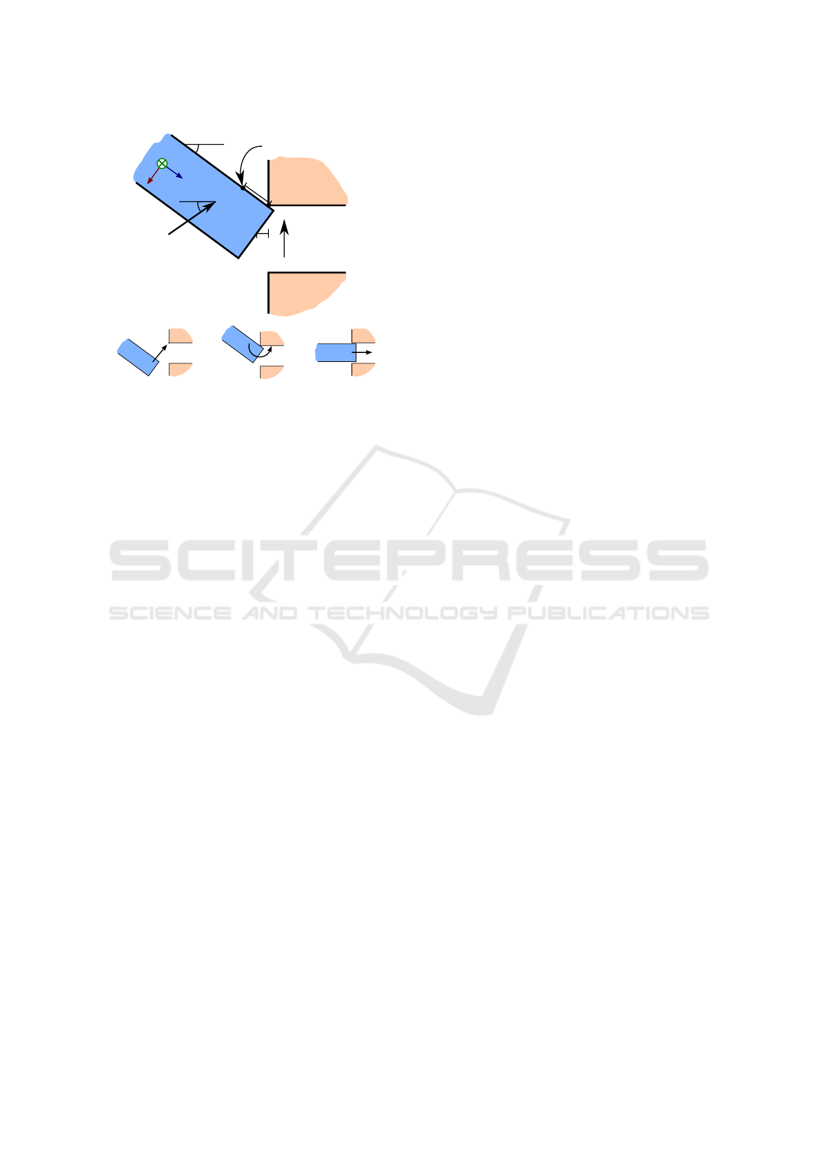
x
φ
y
z
x
y
θ
Rotation Point
Initial
movement
Compliance
direction of
brass fitting
1
2
3
Figure 3: The PiH action. Top: The four parameters defin-
ing the PiH parameters. Bottom: The three movements of
the PiH action as defined by the four parameters.
the peg touches the hole. The location of the peg at
this point is defined by the perpendicular distance x
from the hole to the centre of the end of the peg. Sec-
ondly, a circular movement of the peg is made around
the “Rotation Point” defined by the parameter y. This
movement ends when the peg is perpendicular to the
surface of the hole. The last movement is a linear in-
sertion of the peg into the hole.
From the above description, the ideal relative path
between the peg and hole is calculated for the chosen
parameter set. This path can then be executed in sim-
ulation and on the real world setup under the influence
of part variations and process uncertainties.
It is considered a success if the peg is placed into
the hole after the execution ends; otherwise a failure
(e.g. if the peg gets stuck by hitting the brass fitting).
This evaluation is automatically labelled in simulation
but manually done for real world experiments.
Compliance between peg and hole is an important
factor to prevent high contact forces which can dam-
age both robot, equipment and item when not having
sensorial feedback. This compliance is utilised under
the circular movement to overcome the part variations
and process uncertainties. In the test case, compliance
is present by letting the brass fitting move upwards in
the feeder system following the direction of compli-
ance (see Figure 3).
The ranges of the parameters are chosen in ad-
vance of the experiment and define the boundaries in-
side which the iterative learning method can perform
the search. In this work, we will limit ourselves to the
investigation of the three parameters x, θ and ϕ, while
fixing the fourth parameters y to 10 mm. The ranges
of the parameters are manually chosen to [−5; 5]mm,
[0;30]
◦
and [0; 45]
◦
for x, θ and ϕ respectively based
on prior knowledge of the test case. The limitation to
three parameters makes visualisation and inspection
easier to handle and decreases the computation time.
The method is not limited to three or fewer parame-
ters in general, but the subject of dimensional scaling
has to be further investigated.
5.2 The Dynamic Simulator
The quantity of experiments needed for a reliable es-
timation often makes it infeasible to use real world
experiments. In addition, simulations are typically
easier to setup (given a usable framework) and can
provide automatic process evaluation, which is often
difficult in the real world. Therefore, we use simula-
tion as a tool for finding good parameters in this work.
The choice of simulator engine relies on its ability
to make realistic dynamic simulations in high quan-
tities. AnonymousEngine (Thulesen and Petersen,
2016) is such a simulator.
To make it possible for the iterative learning
method to deal with part variations and process un-
certainties, corresponding perturbations are added to
the relevant workpieces for each simulation. Note that
the simulator itself is deterministic, but the learning
method does see a non-deterministic process due to
the added perturbations.
Each perturbation is drawn from a predefined den-
sity distribution reflecting the part variations and pro-
cess uncertainty in the real assembly process. In our
PiH test case translational perturbations are made in-
dependently along the x- and y-axis of the peg (see
Figure 3), both drawn from a normal distribution with
standard deviation of 0.35 mm, where the confidence
level is chosen to 95% (z = 1.96). If this value ex-
ceeds plus/minus one standard deviation a new draw
is made since extreme values do not occur in the real
world PiH test case. This results in a maximum trans-
lation of ±0.49mm.
5.3 Experiment Choices
In this section we select first the type of kernel, then
the bandwidth matrix used by the KDE representation
is found, and lastly a discretisation of the parameter
space is made.
5.3.1 The Kernel Type and Bandwidth
In this work we choose to use a diagonal multi-
normal (Gaussian) kernel to reduce complexity when
the optimal bandwidth has to be found. This choice
does assume independence between the parameters
ICINCO 2016 - 13th International Conference on Informatics in Control, Automation and Robotics
172
but leaves only three elements (one for each of chosen
parameters) for which the optimal values should be
found instead of six elements when using a full band-
width matrix. Note that the matrix must be symmetric
and positive definite.
The bandwidth matrix used in the case is trans-
ferred from a previous similar case. We do believe
that a suitable kernel size can be transferred from sim-
ilar cases. This means that simulations made for opti-
mising the kernel are reused and omitted when setting
up a similar case.
The Cross-Validation (CV) error function was
used (see Section 3.3.2) to find a suitable bandwidth
matrix in the previous case. The error function was
minimised using the Coordinate Descent algorithm to
find the optimal bandwidth matrix, H. The samples
were drawn randomly from a uniform distribution
over the entire parameter space, S. The minimisation
was performed five times and each time with 5000
randomly chosen samples. This was done to account
for both the stochastic behaviour of the process and
to ensure sufficient coverage of the parameter space.
The average of the five minimisations equates to:
H = diag
h
x
= 0.20 , h
θ
= 0.93 , h
ϕ
= 8.18
(11)
5.3.2 Discretisation of the Parameter Space
To have a discretisation which both covers the space
and where the chosen kernel can influence neighbour-
hood points, it was decided to have 1.5 standard devi-
ations between each of sample points. Based on (11)
and the parameter ranges this leaves a discretisation
of 35, 23 and 5 steps for the three parameters x, θ and
ϕ respectively, which results in a grid consisting of
4025 sample points.
6 EXPERIMENTS AND RESULTS
This section shows how the iterative learning method
can be used to find promising parameter sets by fast
reduction of the parameter space. Section 6.1 com-
pares the performance of the iterative learning method
using Kernel Density Estimation with Wilson Score
and simple Na
¨
ıve Sampling. In Section 6.2 a promis-
ing parameter set found by the learning method with
KDE is tested on a real world setup.
6.1 Applying the Iterative Learning
Method
In this section, we first apply the iterative learning
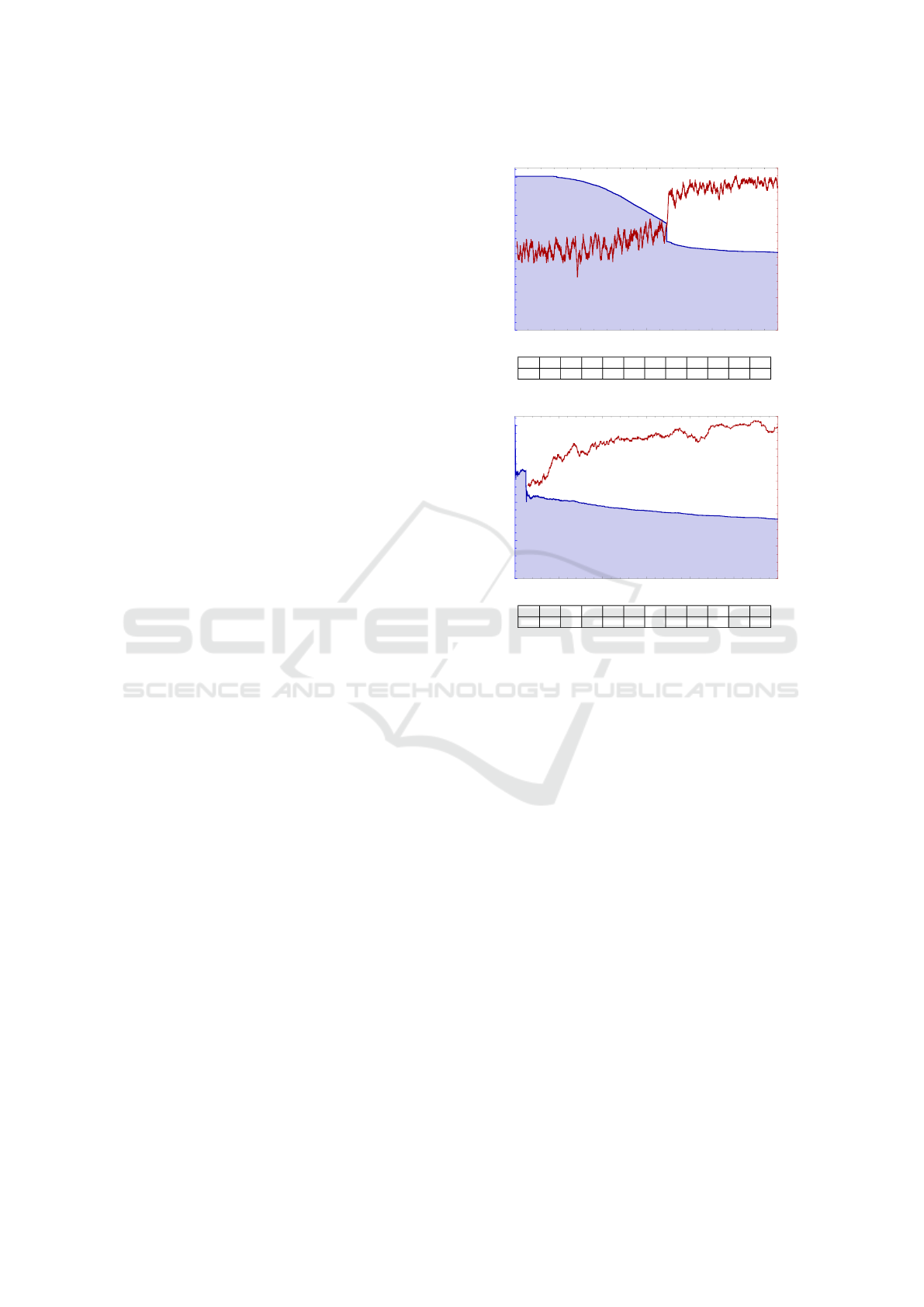
method with WS and find that the number of samples
0 5000 10000 15000 20000
0
1000
2000
3000
4000
Iterations
Samples
Wilson Score
0
20
40
60
80
100
Performance [%]
Ite.
1 2000 4000 6000 8000 10k 12k 14k 16k 18k 20k
Samp.
4025 4025 3967 3801 3508 3108 2267 2139 2082 2055 2033
0 500 1000 1500 2000 2500 3000
0
1000
2000
3000
4000
Iterations
Samples
Kernel Density Estimation
0
20
40
60
80
100
Performance [%]
Ite.
1 300 600 900 1200 1500 1800 2100 2400 2700 3000
Samp.
4025 2135 2039 1929 1842 1780 1723 1659 1626 1599 1560
Figure 4: Blue graph: The number of samples still in con-
sideration after global exclusion when applying the iterative
learning method. Red graph: The performance of the learn-
ing method by the percentage of successful experiments
within the past 150 iterations. The table below show the
number of samples of samples still in consideration at the
given iteration. Top: using WS representation for 20.000
iterations. Bottom: using KDE representation for 3000 iter-
ations. Note the different scales of the horizontal axes.
needed is high compared to KDE where the neigh-
bour samples are taken into account. Afterwards, we
study the performance of the KDE estimate by com-
paring the obtained regression values with a simple
NS. Lastly, a set of action parameters is chosen for
the real world experiment.
6.1.1 Comparison Between the WS and KDE
Data Representations
A comparison between WS and KDE is shown in Fig-
ure 4. The blue plot and the table below each graph
expresses the number of sample points still in con-
sideration after the global exclusion by the iterative
learning method. The red graph shows the perfor-
mance of the learning method by the percentage of
successful experiments within the last 150 iterations.
For WS, the number of samples slowly decreases
Online Action Learning using Kernel Density Estimation for Quick Discovery of Good Parameters for Peg-in-Hole Insertion
173

during the iterations. The large exclusion of 470 sam-
ples after 11541 iterations occurs since these samples
suddenly do not overlap with the current best sam-
ple. Afterwards, the decrease in the number of sam-
ples still in consideration levels off. This shows that a
large number of iterations are used for exploring the
parameter space in the beginning, after which the fo-
cus is turned towards the most promising samples in
the parameter space. Compared to the WS results it is
clear that KDE quickly excludes what is believed to
be the bad regions of the sample space, and hereafter
only spends time refining the knowledge in the more
promising region with further exclusions.
From the performance measure, it can be seen
that WS at 11668 iterations reaches 80% performance
(90% at 12773) which for KDE happens just before
iteration 633 (90% at 1610). When examining the
number of samples still in consideration, WS requires
more than 20000 iterations to reduce the number of
samples to 2000 which by KDE achieved after just
722 iterations. Both of these observations show that
KDE is faster than WS
2
.
In previous experiments, the iterative method us-
ing KDE was applied to an analytic function used as
ground truth. The analytic function describes a PiH
case closely related to the one presented in this pa-
per. The result showed that the ten sample points with
the highest value estimated by KDE within 1000 iter-
ations were located on a point where the ground truth
had a success probability above 99%. This clearly in-
dicates that the presented learning method using KDE
is able to find promising regions of parameter space.
Since WS is observed to be five times slower than
KDE in the reduction of samples, the WS representa-
tion will be omitted in future comparisons.
6.1.2 Comparing KDE Representation and
Na
¨
ıve Sampling
For comparing the KDE regression estimate NS is
used. From NS, the normal binomial mean and confi-
dence interval is calculated for each sample point and
used as an estimate on the true value. Each point is
sampled 100 times which results in a total of 402500
simulation runs.
In Figure 5 two cross-sectional views of the re-
gression value at ϕ equal 0.0
◦
and 11.25
◦
for both
KDE (left column) and NS (right column) are shown.
These two views are highlighted since only approach
angles (ϕ) below 20
◦
are usable in real world due to
2
We do in the comparisons not consider the 5000 sam-
ples used for finding the optimal kernel size by Cross-
Validation (CV). A suitable kernel size can be chosen from
knowledge obtained in previous similar cases.
-4 -2 0 2 4
0
5
10
15
20
25
30
x [mm]
theta [°]
KDE: regression for phi=0.00°
0
0.2
0.4
0.6
0.8
1.0
-4 -2 0 2 4
0
5
10
15
20
25
30
x [mm]
theta [°]
Naive: regression for phi=0.00°
0
0.2
0.4
0.6
0.8
1.0
-4 -2 0 2 4
0
5
10
15
20
25
30
x [mm]
theta [°]
KDE: regression for phi=11.25°
0
0.2
0.4
0.6
0.8
1.0
-4 -2 0 2 4
0
5
10
15
20
25
30
x [mm]
theta [°]
Naive: regression for phi=11.25°
0
0.2
0.4
0.6
0.8
1.0
Figure 5: Comparison of the success probability between
the KDE and NS results. Each of the four plots represents a
cross-sectional view of the parameters x and θ at a fixed ϕ.
The red and blue dots represent the best sample points found
by NA and KDE respectively. The yellow dots represent
three bad points used for the real world experiment. See
text for more information.
accessibility.
By visual inspection, similarities between NS and
KDE are clearly seen. Please note that NS is not the
ground truth, since only 100 experiments are made in
each sample point. However, NS makes for a good
comparison since the points are not influenced by
smoothing as for KDE.
We compare KDE and NS by finding the best
sample points from KDE and by outlining the 99%
contour line from NS. However, to avoid selecting
close lying points from the KDE result, sample points
within a certain region of the already selected sam-
ple are rejected. In this case, the choice is made to
omit sample points within 2 points of an already se-
lected point for x and θ which corresponds to 0.7 mm
and 3.4
◦
respectively. The angle ϕ is not constrained,
since this parameter is discretised in steps of 11.25
◦
.
Moreover, to avoid border effects also the samples at
x equal −5 mm and 5 mm and at θ equal 0
◦
and 30
◦
are eliminated.
In Figure 5 the best points from KDE and the out-
line of the NS 99% contour line within the two cross-
sectional views are shown. The red line represents the
NS 99% contour line. Note that 300 of the 318 points
within the two 99% contour outline areas have a suc-
cess probability at 99% or above. The remaining 18
points has at least a success probability at 95%. More-
over, 16 points with a success probability at 99% or
above are located outside the contour area due to their
ICINCO 2016 - 13th International Conference on Informatics in Control, Automation and Robotics
174

Table 1: Performance of the ten candidate points found.
Sample Success probability
number KDE [%] Na
¨
ıve [%] Re-sam. [%]
1 100.0 100 ± 0.0 98.8 ± 1.0
2 100.0 100 ± 0.0 98.8 ± 1.0
3 100.0 99 ± 2.0 98.4 ± 1.1
4 100.0 100 ± 0.0 98.8 ± 1.0
5 100.0 100 ± 0.0 98.8 ± 1.0
6 100.0 100 ± 0.0 98.8 ± 1.0
7 100.0 99 ± 2.0 98.6 ± 1.0
8 100.0 100 ± 0.0 98.8 ± 1.0
9 100.0 99 ± 2.0 98.2 ± 1.2
10 100.0 100 ± 0.0 97.0 ± 1.5
sparse appearance. The blue dots represents the ten
best points chosen by KDE while omitting close ly-
ing points.
Figure 5 shows that the ten candidate points sug-
gested by KDE all lies with the 99% contour area
from NS. Moreover, these points are mostly located
in the middle of the contour area. Seven of the ten
points are located on points from the NS point with
100% success probability, while the remaining three
points are located on a NS point with a 99% success
probability. This clearly indicates that KDE has found
a true good region, and that KDE suggests the points
pushed away from bad regions and into the middle of
a success region even if a plateau appears as for this
case.
All ten sample points chosen from KDE re-
sults have an estimated KDE regression value above
99.99%. A comparison of these values with the val-
ues obtained from NS are shown in Table 1.
6.1.3 Refining the Promising Parameter Sets
Before real world experiments can be carried out, one
parameter set needs to be selected. However, just se-
lecting the sample point with the highest regression
value among the ten candidates suggested by the it-
erative learning method might not be the best choice.
The regression values obtained by the iterative learn-
ing method with KDE are influenced by the kernel
smoothing, and do therefore not reveal the true value.
A simple way to deal with this problem is to fur-
ther test the candidate points by simulations to re-
veal a more reliable estimate on the true regression
value. Each of the ten candidate points is re-sampled
500 times with perturbations, from which the bino-
mial mean and confidence interval have been calcu-
lated (see the “Re-sam.” column in Table 1). This
further testing of these good candidates is only possi-
ble due to the reduction of sample points, and would
have been infeasible to make for all sample points.
Figure 6: From left to right: Three “bad” sample points and
the selected “good” point from two different angles. For
the “bad” points the peg either collides with the brass fitting
below or above the hole and does therefore fail. The images
in the right column show a success for the “good” point.
Even though each point in the re-sampling was
sampled 500 times, it is impossible to distinguish the
ten points by statistical certainty. Moreover, the com-
parison between the NS and the re-sampling clearly
shows that only taking 100 samples in each point are
not enough for result to be reliable. This fact just
stresses the need for a fast reduction of the parame-
ter space.
The re-sampling shows that six of the ten candi-
date points all have obtained the highest success prob-
ability at 98.8%, and therefore sample number five is
randomly chosen for the test on the real world setup.
6.2 Real World Results
In this section real world experiments are carried out
based on the results from the previous section. The
simulator is rather conservative compared to the real
world by not implementing compliance between grip-
per and pipe, which may be enough to raise the suc-
cess probability sufficiently.
Besides executing the selected “best” sample
point 100 times also several “bad” sample points are
tested. These points were chosen manually to show
that the promising region found by the iterative learn-
ing method in simulation also aligns with the real
world case. These “bad” points are shown in yellow
in Figure 5.
The three “bad” samples points were tried out
once each. As Figure 6 shows these sample points
fail to succeed since the peg collides with the brass
fitting either below or above the hole. The figure also
shows that the “good” sample point selected for ex-
ecution succeeds. Recall that the approach angle is
either 0
◦
or 11.25
◦
for all four points.
After this observation the selected “best” sample
point found by the iterative learning method using
KDE was tested. The experiments were made by cir-
culating between ten different pipes and brass fittings
to introduce part variations. The real world test of
the selected “best” sample point was carried out 100
times with a success rate of 100%. The number 100
was chosen as sufficient to show that good parame-
Online Action Learning using Kernel Density Estimation for Quick Discovery of Good Parameters for Peg-in-Hole Insertion
175

ter sets can be chosen from simulation and executed
in real world. A longer test should be conducted to
verify that the selected set of parameters is robust to
small changes occurring over the lifetime of the setup.
7 SUMMARY
In this paper we proposed an iterative learning method
which differs from other methods by being able to
take into account part variations and process uncer-
tainty. This property is very important to find ac-
tion parameters which are guaranteed to succeed ev-
ery time in precision demanding assemblies as for the
Peg-in-Hole task discussed in this paper.
Experiments showed that our iterative learning
method is able to quickly reduce of the parameter
space using Kernel Density Estimation which takes
the neighbourhood region into account. This ap-
proach was faster than both neighbourhood indepen-
dent representation Wilson Score and simple Na
¨
ıve
Sampling. It was shown that KDE is able to find good
sample points much faster than a representation which
individually estimates the success probability of each
of the sample points.
In the conducted experiment, promising sets of pa-
rameters were found by the iterative learning method
using KDE through simulation. From the knowledge
obtained by the method a promising sample point was
selected for a real world Peg-in-Hole experiment. The
experiment was repeated 100 times with a success
rate of 100%. Moreover, real world experiments also
showed that the iterative learning method converged
successfully towards the promising region of the pa-
rameter space.
Future work will study the effect of different band-
width matrices which might speed up the iterative
learning method and potentially improve the quality
of the points found. The result when applying the it-
erative learning method with KDE showed both an
over- and underestimation of the regression values in
certain spots. These peak spots are probably an ef-
fect of a too narrow kernel. An adaptive kernel size
should also be investigated since the bandwidth ma-
trix is known to change with the number of samples.
ACKNOWLEDGEMENTS
This work was supported by The Danish Council for
Strategic Research through the CARMEN project.
REFERENCES
Agresti, A. and Coull, B. A. (1998). Approximate Is Better
than ”Exact” for Interval Estimation of Binomial Pro-
portions. The American Statistician, 52(2):119–126.
Auer, P., Cesa-Bianchi, N., and Fischer, P. (2002). Finite-
time analysis of the multiarmed bandit problem.
Mach. Learn., 47(2-3):235–256.
Bodenhagen, L., Fugl, A., Jordt, A., Willatzen, M., An-
dersen, K., Olsen, M., Koch, R., Petersen, H., and
Kruger, N. (2014). An adaptable robot vision system
performing manipulation actions with flexible objects.
Automation Science and Engineering, IEEE Transac-
tions on, 11(3):749–765.
Brochu, E., Cora, V. M., and de Freitas, N. (2010). A
tutorial on bayesian optimization of expensive cost
functions, with application to active user model-
ing and hierarchical reinforcement learning. CoRR,
abs/1012.2599.
Buch, J., Laursen, J., Sørensen, L., Ellekilde, L.-P., Kraft,
D., Schultz, U., and Petersen, H. (2014). Apply-
ing simulation and a domain-specific language for an
adaptive action library. In Simulation, Modeling, and
Programming for Autonomous Robots, pages 86–97.
Springer International Publishing.
Deisenroth, M. P., Neumann, G., and Peters, J. (2011). A
survey on policy search for robotics. Foundations and
Trends in Robotics, 2(1–2):1–142.
Detry, R., Kraft, D., Kroemer, O., Bodenhagen, L., Peters,
J., Kr
¨
uger, N., and Piater, J. (2011). Learning grasp
affordance densities. Paladyn, 2(1):1–17.
EU Robotics aisbl (2014). Robotics 2020 multi-annual
roadmap for robotics in europe.
Even-Dar, E., Mannor, S., and Mansour, Y. (2006). Ac-
tion elimination and stopping conditions for the multi-
armed bandit and reinforcement learning problems.
The Journal of Machine Learning Research, 7:1079–
1105.
Gams, A., Petric, T., Nemec, B., and Ude, A. (2014). Learn-
ing and adaptation of periodic motion primitives based
on force feedback and human coaching interaction. In
Humanoid Robots (Humanoids), 2014 14th IEEE-RAS
International Conference on, pages 166–171.
H
¨
ardle, W., Werwatz, A., M
¨
uller, M., and Sperlich, S.
(2004). Nonparametric and semiparametric models.
Springer Berlin Heidelberg.
Heidrich-Meisner, V. and Igel, C. (2009). Hoeffding and
bernstein races for selecting policies in evolutionary
direct policy search. In Proceedings of the 26th An-
nual International Conference on Machine Learning,
ICML ’09, pages 401–408. ACM.
Ijspeert, A. J., Nakanishi, J., Hoffmann, H., Pastor, P., and
Schaal, S. (2012). Dynamical movement primitives:
Learning attractor models for motor behaviors. Neural
Computation, 25(2):328–373.
Jørgensen, T. B., Debrabant, K., and Kr
¨
uger, N. (2016).
Robust optimizing of robotic pick and place opera-
tions for deformable objects through simulation. In
Robotics and Automation (ICRA), 2016 IEEE Inter-
national Conference on. (accepted).
ICINCO 2016 - 13th International Conference on Informatics in Control, Automation and Robotics
176

Li, B., Chen, H., and Jin, T. (2014). Industrial robotic as-
sembly process modeling using support vector regres-
sion. In Intelligent Robots and Systems (IROS 2014),
2014 IEEE/RSJ International Conference on, pages
4334–4339.
Park, D., Kapusta, A., Kim, Y. K., Rehg, J., and Kemp,
C. (2014). Learning to reach into the unknown: Se-
lecting initial conditions when reaching in clutter. In
Intelligent Robots and Systems (IROS 2014), 2014
IEEE/RSJ International Conference on, pages 630–
637.
Robotics VO (2013). A roadmap for U.S. robotics from
internet to robotics.
Ross, S. M. (2009). Introduction to Probability and Statis-
tics for Engineers and Scientists. Acedemic Press, 4th
edition.
Silverman, B. W. (1986). Density estimation for statistics
and data analysis, volume 26. Chapman & Hall/CRC
press.
Sutton, R. S. and Barto, A. G. (1998). Reinforcement learn-
ing: An introduction, volume 28. MIT press.
Tesch, M., Schneider, J. G., and Choset, H. (2013). Expen-
sive function optimization with stochastic binary out-
comes. In Proceedings of the 30th International Con-
ference on Machine Learning, ICML 2013, Atlanta,
GA, USA, 16-21 June 2013, pages 1283–1291.
Thulesen, T. N. and Petersen, H. G. (2016). RobWork-
PhysicsEngine: A new dynamic simulation engine for
manipulation actions. In Robotics and Automation
(ICRA), 2016 IEEE International Conference on. (ac-
cepted).
Williams, R. J. (1992). Simple statistical gradient-following
algorithms for connectionist reinforcement learning.
Machine Learning, 8(3):229–256.
Yang, Y., Lin, L., Song, Y., Nemec, B., Ude, A., Buch, A.,
Kr
¨
uger, N., and Savarimuthu, T. (2015). Fast pro-
gramming of peg-in-hole actions by human demon-
stration, pages 990–995. IEEE.
Online Action Learning using Kernel Density Estimation for Quick Discovery of Good Parameters for Peg-in-Hole Insertion
177
