
A WSN-based, RSS-driven, Real-time Location Tracking System
for Independent Living Facilities
Pawel Gburzynski
1,2,4
, Wlodek Olesinski
2
and Jasmien Van Vooren
3
1
Vistula University, Computer Science, Warsaw, Poland
2
Olsonet Communications Corporation, Ottawa, Ontario, Canada
3
Alphatronics, Lokeren, Belgium
4
Sendronet, Wierzchowo, Poland
Keywords:
Wireless Sensor Networks, Real-time Location Tracking, Ad-hoc Networking.
Abstract:
We present an indoor location tracking system (RTLS) based on a wireless sensor network (WSN) where
the received signal strength (RSS) readings collected by immobile nodes (Pegs) from mobile (tracked) nodes
(Tags) are translated into location estimates for the Tags. The process employs a database of samples pre-
viously collected from known locations; thus, the scheme falls into the category of profile-based solutions,
with RSS readings being the only kind of input to the estimator. Compared to other schemes hinged on the
same general idea, the novelty of our approach consists in systematically taking advantage of multiple transmit
power levels at the Tags. This allows us to effectively emulate RFID-type of operation, when a nearby Peg
can authoritatively identify the location by perceiving a weak signal from the Tag (indicative of the Tag’s im-
mediate proximity), while otherwise falling back to elaborate fitting of multiple readings (collected by several
Pegs) to produce a (possibly approximate) location estimate. The location service of our network is an add
on to its other duties which consist in providing connectivity within an independent living (IL) facility for the
purpose of inconspicuously monitoring the patients, detecting anomalies, signaling alarms, and so on.
1 INTRODUCTION
The work reported in this paper is the offspring of
our earlier study (Haque et al., 2009) evolved into a
collaborative effort undertaken by Olsonet
1
and Al-
phatronics
2
aimed at creating a comprehensive WSN
to outfit a number of IL facilities in Belgium. The
primary goal of the WSN is to provide an an open-
ended, low-bandwidth, self-contained, flexible com-
munication platform for detecting and signaling vari-
ous events, usually related to the well being of the IL
patients, e.g., see (Boers et al., 2010).
1.1 Previous Work
Early attempts to transform RSS readings into loca-
tions (Christ et al., 1993) were based on interpreting
RSS as a function of distance between the transmit-
ter and the receiver. While some generic models of
this kind have been claimed to well capture the statis-
1
http://www.olsonet.com
2
http://www.alphatronics.be
tics of “typical” indoor environments, e.g., for simu-
lation (Mart´ınez-Sala et al., 2005), their blanket ap-
plication in RTLS has not met with success. Thus, if
used at all, they were augmented with some heuristics
or tweaks, accounting at least for some standard ob-
stacles of a permanent nature, e.g., walls (Christ et al.,
1993).
The whimsical nature of RSS indications inspired
approaches based on other features of RF signals.
The most popular among them can be categorized
as: Time of Flight (TOF), Time of Arrival (TOA),
Time Difference of Arrival (TDOA), Angle of Ar-
rival (AOA), and Near-Field Electromagnetic Rang-
ing (NFER). The first three among them (Deak et al.,
2012) require a precise measurement of the propaga-
tion time between the sender and the receiver. With
AOA, the measured entity is the angle from the re-
ceiver towards the sender; the scheme is often com-
bined with TOA (Venkatraman and Caffery Jr, 2004)
to mitigate the impact of obstacles. The NFER tech-
nique (Schantz, 2007) relies on measuring the differ-
ence in phase between the electric and magnetic com-
ponents of the electromagnetic field (at the receiver)
64
Gburzynski, P., Olesinski, W. and Vooren, J.
A WSN-based, RSS-driven, Real-time Location Tracking System for Independent Living Facilities.
DOI: 10.5220/0005959000640071
In Proceedings of the 13th International Joint Conference on e-Business and Telecommunications (ICETE 2016) - Volume 1: DCNET, pages 64-71
ISBN: 978-989-758-196-0
Copyright
c
2016 by SCITEPRESS – Science and Technology Publications, Lda. All rights reserved

which tends to depend on the distance.
All the above techniquesrequire specific hardware
features which are not needed for “normal” RF com-
munication and often get in the way. This basically
means that an RTLS must be devised and deployed
as a separate system using its own dedicated hard-
ware. For example, NFER devices operate within the
AM band (530-1710 kHz) which is exotic from the
viewpoint of contemporary communication network-
ing. The most successful time/angle-based devices
operate in Ultra Wide Band (UWB) (Kempke et al.,
2015), to mitigate the effect of reflections, and, at
least in our experiments, exhibit significantly lower
communication range (combined with a much higher
power consumption) compared to popular ISM-based
modules. All of them work reliably within LOS en-
vironments, where they are truly unbeatable in terms
of accuracy, but any obstacles (especially those caus-
ing unbypassable reflectons) tend to significantly af-
fect the readings.
1.2 The Prerequisites and the Problem
The WSN constituting the basis for our system con-
sists of two types of nodes which will be referred to
as Tags and Pegs (Gburzy´nski and Olesi´nski, 2008).
Pegs are the anchors, i.e., their locations are ba-
sically fixed, while Tags are mobile. Both node
types are built around the same RF module which
is CC430F6137 by Texas Instruments (Texas Instru-
ments, 2014). The device operates within the ISM
band (which is 816 MHz for the system at hand).
The Pegs jointly form the actual ad-hoc net-
work whereby (relevant) packets are forwarded, us-
ing TARP (Gburzy´nski et al., 2007), to a central sink
dubbed the master. The nominal baud rate for RF-
communication is 38,400 bps. The maximum (pay-
load) packet length is 54 bytes. The master interacts
with the OSS over a USB connection to a workstation
computer. A Tag communicates with the system via
Pegs.
Unlike (Haque et al., 2009), by location we do not
understand a point, say in 3-d, to be pinpointed with
some desirable accuracy, but a named area (or space)
whose size and shape generally depend on the con-
text. For example, its granularity may correspond to a
room, or even an apartment or a corridor, if it happens
to be satisfactory from the viewpoint of the operator.
Generally, the system is not expected to be 100% re-
liable. In particular, it may offer a number of alter-
native (suspect) locations ranking them according to
some measure of likelihood.
Note that the above assumptions shed a new light
on the comparison of the RSS-based approach to lo-
cation tracking with the other techniques mentioned
in Sec. 1.1. For example, if we switched to a TOA-
capable RF-module, we would not be able to take the
full advantage of its capability, because the applica-
tion where such a device truly excels, i.e., locating the
Tag precisely within a (potentially large) room outfit-
ted with several (at least three, and preferably four)
anchors-Pegs deployed within the Tag’s LOS (say, in
the corners at the ceiling), is of no interest to us. In-
stead, we want to be able to tell apart the different
rooms (or blocks of rooms) for which the TOA ap-
proach doesn’t work too well, because of the impos-
sibility of LOS communication.
2 THE TRACKING SYSTEM
A tracked Tag emits at its discretion so-called location
bursts which are series of short packets sent back-to-
back at different power levels. In the present system,
a location burst consists of 32 packets, 4 packets per
each of eight discrete transmit power levels numbered
0 through 7. Any Peg receiving any packets of a burst
prepares a location report and expedites it to the mas-
ter.
The transmit power levels have been calibrated ex-
perimentally, such that the perceived difference be-
tween two adjacent levels is about 5 dB. The value of
RSS directly translates into the received power level
in dBm quantized into steps of 0.5 dBm (plus some
fixed offset). We do not assume that the location
bursts are issued at any specific intervals. Generally,
those intervals can be long, so we do not incorpo-
rate history (previous estimates) into the tracking al-
gorithm. It is obvious that making the bursts periodic
(and frequent) and accounting for the history of recent
estimates will tend to improve the accuracy of estima-
tion. For example, (Ni et al., 2004) discuss a remark-
ably accurate scheme achieved with just one anchor
node (a WiFi access point) plus some profiling, some
modeling, and a rather heavy reliance on the history
of previous estimates. Another possibility is to apply
prediction models for traffic (Cho and Kwon, 2016)
which, considering the specifics of the target environ-
ment, is likely to further reduce the uncertainty in po-
sition. This work has been left as a natural goal for
the future.
The only relevant kind of data arriving at the loca-
tion server is a sequence of burst reports from Pegs.
Formally, a report is a 4-tuple R = (P,T,r,V) where
P is the Peg Id, T is the Tag Id, r is a by-Tag serial
number identifying the burst, and V = (v
0
,. .. ,v
7
) is
the RSS vector consisting of eight single-byte values
representing the averaged RSS readings for the eight
A WSN-based, RSS-driven, Real-time Location Tracking System for Independent Living Facilities
65

power levels (note that a Peg may receive up to four
packets per level). A value of zero (which can never
be a legitimate RSS reading) means that no packets
corresponding to the given power level have made it
to the Peg.
2.1 Profiling
The tracking is driven by a database of samples col-
lected from known locations. For this, the area is pro-
filed and the reports collected during this process are
stored in the database along with their locations. Dur-
ing the actual tracking, the location reports are com-
pared against the profile samples. Roughly speaking,
the Tag’s location is estimated as the one attributed
to those profile samples from the database that best
match the tracking reports.
Formally, locations are identified by numbers re-
ferred to as internal location identifiers. The OSS is
responsible for mapping those internal identifiers to
external locations, i.e., descriptors presented to the
human operator. A single external location may cor-
respond to a number of internal locations acting as
their union. For example, partitioning a geometri-
cally compound location into smaller (regular) frag-
ments may lead to a simpler, less complex computa-
tionally, and more representative (reliable) coverage
of the smaller subareas with their individual sets of
samples. Also, overlapping internal locations may
represent the same area sampled in different ways,
e.g., as to capture some modal feature of the Tag: its
particular elevation above the floor, orientation, etc.
The aim of the profiling procedure is to collect
samples from known (internal) locations. The way
the server guesses at the location of a tracked Tag
(Sec. 2.2) suggests these recommendations for sam-
ple collection.
1. The (internal) locations should be reasonably sim-
ple, preferably rectangular and close to squares.
2. The number of samples per (internal) location
need not be large, but the samples should be com-
plete and reliable; consequently, it makes sense to
combine/average multiple samples taken from the
same point of a given location.
The server offers hooks to facilitate profiling. Having
moved to the point from where a sample is to be col-
lected, the user anchors the Tag. This operation tells
the server to assume that any burst reports referring
to the Tag should now be attributed to a sample. The
sample is identified by the location Id and the collec-
tion point Id, the latter being a location-relative mark
whose purpose is to tell apart different samples col-
lected from the same location. A button press on the
Tag will trigger a location burst. A report from that
burst arriving at the server will be added to the sam-
ple. Multiple reports from the same Peg are merged,
i.e., the RSS vector entries of the sample are averaged
using this formula:
v
i( j)
= v
i
× α+ v
i( j−1)
× (1− α) (1)
where v
i( j)
is the updated value of entry i in the av-
eraged RSS vector, v
i( j−1)
is the previous value of
that entry, v
i
is the new reading (from the newly re-
ceived report), and α is a parameter (with the default
value of 0.3). The update does not occur when v
i
= 0,
i.e., the report has no RSS value for the given power
level. This exponential moving average ensures that
new samples tend to override old ones, so previously
profiled locations can be easily (and selectively) re-
profiled later.
Formally, a sample is a triplet S =
(L,s,{P
i
,V
i
}
k−1
i=0
) where L is the (internal) loca-
tion identifier, s is the sample identifier (relating
to the collection point within the location), and the
third element is the set of pairs: Peg Id (P
i
) and
the corresponding RSS vector (V
i
), representing the
burst reports that have contributed to the sample (k is
the number of different Pegs that have received the
bursts).
2.2 The Estimation Algorithm
The server stashes the arriving burst reports on a per-
Tag basis, aggregating them into a tracking set, i.e.,
sufficiently many reports (for the given Tag) to use
them for location estimation. A stashed report is time-
stamped with its arrival time.
Let us focus on some Tag T. Suppose that a new
report R = (P,T,r,V) arrives at the server at time t.
The server examines the current set of stashed reports
for T and, for each report R
i
= (P
i
,T,r
i
,V
i
) performs
these actions:
1. Let t
i
be the time stamp of R
i
. If r
i
6= r andt
i
+δ
s
<
t, then R
i
is deemed obsolete and discarded from
the stash. The default value of δ
s
is 4 seconds.
2. If P
i
= P, then the new report augments the
stashed one. The elements of V
i
are updated in
R
i
according to formula 1, the time stamp of R
i
is
refreshed to t, the new report R is discarded. Then
the next report from the stash is taken until all the
reports have been examined.
3. If all stashed reports have been processed, and P
hasn’t matched any P
i
in step 2, the new reading
is added to the stash with time stamp t.
After completing the above loop, the server is ready to
attempt a location estimation, provided that the stash
DCNET 2016 - International Conference on Data Communication Networking
66

contains at least K = 3 reports. As the server never
knows when the last report for a burst is going to ar-
rive, it delays the attempt for δ
e
= 3 seconds. The
estimation procedure is described below.
We start with the tracking set, i.e., the current col-
lection of stashed reports {R
i
}
M− 1
i=0
, where M is the set
size (M ≥ K) and R
i
= (P
i
,T,r
i
,V
i
). Let v
i,l
denote
the l-th element of vector V
i
. For each power level
l, 0 ≤ l < 8, we construct U
l
as the set of 4-tuples
(P
i
l
,l
,v
i
l
,l
) such that v
i
l
,l
are the three largest elements
of
v
i,l
, over all i, 0 ≤ i < M. Then we discard all
elements from U
l
where v
i
l
,l
= 0. Note that U
l
con-
sists of at most three elements and it can be empty. In
plain words, for each of the eight power levels, we se-
lect from all the stashed reports three with the largest
RSS readings, along with their associated Pegs.
Subsequently, the estimator executes a loop in-
dexed by the power level l starting at l = 0 (the lowest
level) and going up to 7. At any iteration, the estima-
tor maintains the current set of candidate locations C
consisting of pairs (L,r), where L is a location and r
is its inverse rank (or badness). The set is initialized
to “all locations” with the identical ranks of 0. Then
we proceed as follows.
1. Consider iteration l. Its objective is to calculate
a set of candidate locations C
l
with ranks based
solely on U
l
. Then the two sets, C and C
l
, are in-
tersected and their ranks combined. The intersec-
tion will possibly trim down the set in size, while
the new ranks will diversify the likelihoods of the
locations still remaining in the set.
If U
l
is empty, then the iteration is skipped, i.e., C
is unaffected and carried over to the next iteration.
2. If U
l
is nonempty, then C
l
is determined as con-
sisting of those locations that have at least one
sample in the database that includes all the Pegs
from U
l
and a nonzero RSSI entry at level l for
each of those Pegs. The procedure for calculating
the ranks for C
l
is discussed below.
3. An attempt is made to intersect C
l
with the run-
ning set C. If the intersection is empty (which will
also happen when C
l
is empty), the loop is exited
with the last nonempty C. Otherwise, C is set to
the intersection. The new ranks (for those loca-
tions that remain in C) are calculated as the sum
of the old ones and the new ones (from C
l
).
When the loop is terminated, the locations in C are
sorted in the inverse order of their ranks and returned
as the location estimate.
A close match to some samples on low power lev-
els is indicative of proximity to the corresponding
Pegs, so it can be used a reliable shortcut for esti-
mating the Tag’s location. In the most advantageous
case, there will be just one location selected this way,
approaching (passive) RFID-type operation. Should
the identification by low power levels turn out to be
imperfect, then: 1) the higher levels may help the es-
timator trim out some locations, 2) a subtler compar-
ison of the reports to database samples will rank the
candidates, thus offering grounds for selection.
The number of elements in nonempty U
l
can 1, 2,
or 3. In the last case,U
l
can be interpreted as a point in
3-space. Thus we deal with one point q obtained from
U
l
and a set of points Q obtained from the database
samples (one point per sample) selected in step 2 of
the above loop. Those samples are grouped by their
locations. Let Q
L
∈ Q be the subset of Q containing
all those samples selected in step 2 of the algorithm
that are attributed to location L. The rank of location
L is calculated as the Euclidean distance from q to the
minimum convexhull encompassing the points in Q
L
.
With the above approach, a sample, including the
tracking set, is interpreted as a point in some simple
metric space, so it makes sense to talk about the dis-
tance between a pair of samples. One can expect that
when we take two samples, from two different spots
of some location, the RSS readings of the Pegs ap-
pearing in both samples will differ, but as one moves
between the two spots, the transition between the vec-
tors (points) is likely to be smooth. Locally, in the best
of the possible worlds, the transition can be approx-
imated by a straight line connecting the two points,
especially if no better model is available. Given mul-
tiple samples referring to the same location, the lin-
ear approach to interpreting transitions among them
boils down to drawing a polyhedron connecting their
points. As, generally, there is more than one way to
draw such a polyhedron, the most natural representa-
tive of them all is the minimum convex hull encom-
passing all the points. Then, it makes sense to assume
that the interior of that hull represents in a certain way
the location covered by the samples.
The algorithm can be tuned through a number of
parameters. First, the original RSS values can be
rescaled via an interpolation table, e.g., to amplify dif-
ferences in large values (which are more indicative of
proximity to the Peg and, generally, more reliable).
Also, when combining the location ranks (step 3), the
ranks from different power levels can be multiplied by
different factors, e.g., to assign a higher importance to
higher levels.
Although Tags are built as fairly homogeneousde-
vices, some discrepancies in the RF properties of dif-
ferent specimens of Tags are unavoidable. This means
that RSS readings from different Tags obtained under
identical conditions may differ slightly. To compen-
sate for this, when calculating the distance between
A WSN-based, RSS-driven, Real-time Location Tracking System for Independent Living Facilities
67
the tracking point q and the convex hull of Q
L
, the
ranking algorithm may turn q into a segment and cal-
culate the distance from the segment to the hull. Sup-
pose that q = (x,y,z) The segment is obtained as the
set of points Q
s
= {(x+ t,y+ t, z+t)}, −ρ ≤ t ≤ ρ,
where ρ is the tolerance parameter settable on a per-
power-level basis. This simple trick assumes that any
fluctuations in the RF characteristics translate into a
linear shift in the transmit power level. Note that
nonzero ρ will tend to blur the quality of location sep-
aration by hulls, so it has to be selected with care.
3 EXPERIMENTS
3.1 The Test System
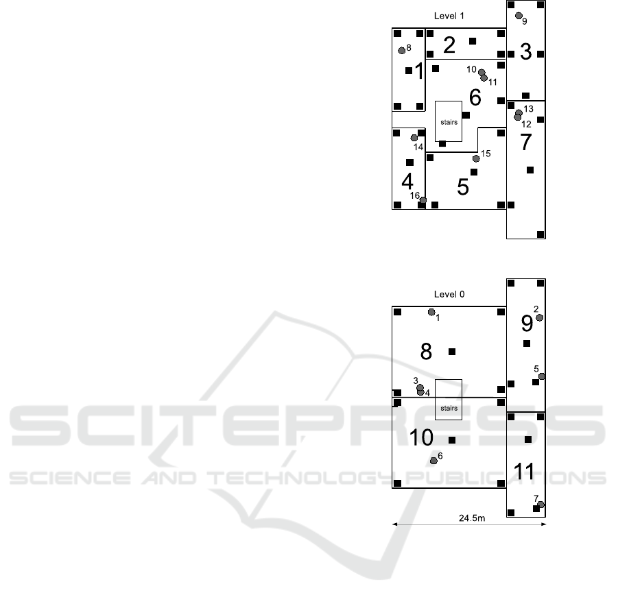
Fig. 1 illustrates a test deployment of our system. The
area consists of two floors: Level 1 comprising of-
fice space with irregular rooms separated by walls,
and Level 0 including a large (exhibition) hall with
some (relatively small) meeting rooms on the south
side. The separation of the two levels into locations
does not strictly follow the division of the area by
walls. In particular, only some walls are drawn at
Level 1 (practically every location encompasses sev-
eral rooms), and the meeting rooms at Level 0 (for-
mally falling into location 10) are not drawn at all.
Also, the separation of the exhibition hall at Level 0
into locations 8 and 10 is purely imaginary. That was
intentional: we wanted to capture (also) the malicious
and fuzzy scenarios where the boundaries between lo-
cation are not clearly demarcated.
The gray circles in Fig. 1 denote the Pegs of our
WSN, 16 of them altogether. Their deployment, while
not completely accidental, is far from perfect. Note
that, e.g., in locations 6 and 8 there are pairs of Pegs
located very close together (Pegs 10, 11 and 3, 4). In
the test network, their deployment has been dictated
by the logistics of other tests carried out in parallel
with the preliminary tests of the location tracking ser-
vice (the co-located Pegs are devices of slightly dif-
ferent types). Consequently, some locations are better
covered than others. For example, the rather difficult
(by its shape) location 11 has only one Peg (7) which,
to make the matters worse, is situated in a corner.
Thus, e.g., one cannot hope that location 11 will be al-
ways perfectly identified. All these problems should
be OK for tests, as long as we understand the limita-
tions.
Figure 1: The test deployment.
3.2 Profiling
The black squares in Fig. 1 mark the collection points
for samples. Within the confines of physical accessi-
bility, we have tried to collect samples from the four
corners of each location as well as from its center. We
shall refer to those points as NW, NE, SW, SE, and C.
Every such a point translates into one sample (being
an average of multiple takes (Sec. 2.1), yielding the
total of 55 samples. For illustration, here is the NW
sample for location 3:
12 0 0 0 0 0 67 75 83
11 0 0 0 0 67 75 78 80
8 0 0 0 0 0 0 82 82
9 82 93 103 112 124 135 148 157
10 0 0 0 0 71 72 87 95
5 0 0 0 0 72 75 80 90
13 0 0 0 0 0 64 74 83
2 0 0 0 69 78 84 92 99
DCNET 2016 - International Conference on Data Communication Networking
68

Each row consists of 9 values: the Peg Id followed by
eight RSS readings for the power levels from 0 to 7
(recall that 0 means “no reading”).
Owing to the inherent lack of reliability in wire-
less communication, and because the packets in loca-
tion bursts are neither acknowledged nor retransmit-
ted, any single report from a location burst can be in-
complete. We have to be prepared for this while track-
ing locations; however, the quality of profiled samples
is important, because a missing reading (or an entire
vector) may affect the interpretation of all tracking
sets. Consequently, a sample is only accepted if it
cannot be improved any more by subsequent bursts
issued from the given collection point, where by im-
provement we mean filling in an entry that was absent
after a previous take.
3.3 Tracking
A low-level RSS entry in a burst report can only be
nonzero when the Tag is relatively close to the Peg.
Thus, some areas are easier to recognize than others.
For example, here is a tracking set collected from the
SW quadrant of location 10:
3 72 77 95 103 113 124 137 145
5 0 0 0 0 0 70 86 96
6 91 95 106 117 128 136 149 157
7 0 0 0 0 80 92 104 109
8 0 0 0 0 0 80 97 103
10 0 0 0 71 78 92 103 109
12 0 0 0 0 0 67 84 93
13 0 0 65 76 90 96 110 115
16 82 94 101 112 124 133 147 154
For power level 0, the only three nonzero entries are
those for Pegs 3, 6, and 16. As it happens, there are
only two samples where 0-level RSS readings for all
those Pegs are present: SW and C for location 10.
Thus, a single location is found in the very first itera-
tion, and the algorithm stops immediately. In fact, the
single report for Peg 6 would suffice, because the two
samples are the only ones that include 0-level read-
ings for that Peg. If the report didn’t make it, then the
two remaining Pegs, 3 and 16, would do. For Peg 16,
there are matching samples in locations 4 (SE, SW,
C), 5 (SW, C), and 10 (SW, C), and for Peg 3, the
samples are in locations 8 (SW) and 10, the only lo-
cation shared by them being 10.
The answer produced by the algorithm is the last
set C (see Sec. 2.2) presented as a list sorted by the
location ranks. Recall that, as calculated by the algo-
rithm (after the last iteration), those ranks are reverse,
so they represent “badness” rather than “goodness” of
a location. Before presentation, they are transformed
into a positive measure of goodness as follows. Let
r
i
, i = 0,... ,n − 1 be the badness of the i-th location
from the list. Let a = (
∑
n−1
i=0
r
i
)/n be the average of
those values. Let g
i
= 1/(r
i
+ a) and S =
∑
n−1
i=0
g
i
. Set
h
i
= (g
i
/S) × 100 and return h
i
as the goodness mea-
sure of location i. Note that all h
i
values add to 100
(so they can be viewed as percentages) and lower val-
ues of r
i
translate into higher values of h
i
. For the
above (easy) estimation case, the server returns a triv-
ial list consisting of the pair (10, 100), i.e., location
10 has been identified as a single candidate with the
goodness rank of 100.
For a more challenging case, here is a tracking
set obtained from a Tag within the NE annex of lo-
cation 5:
5 0 0 0 0 0 70 88 94
7 0 0 0 0 0 83 97 103
9 0 0 0 0 0 0 68 76
10 0 0 0 0 0 0 63 75
12 0 0 0 0 73 85 97 106
13 0 0 62 71 83 96 105 109
16 0 0 0 0 0 75 80 96
The first non-zero power level is 2 with a single report
(Peg 13). In the first stage of the iteration for this
power level, all the samples with a reading for Peg 13
and power level 2 are identified. This brings in the
following list:
1 < 59> < 68> < 68>
2 < 65>
3 < 60> < 81>
4 < 69> < 69> < 58>
5 < 65> < 91> < 67> < 75> < 72>
6 < 61> < 78> < 72> < 72>
7 <109> <103> < 60> < 83> < 60>
8 < 65>
9 < 59> < 73>
10 < 69>
11 < 77> < 69> < 74> < 65>
The first number in each line is the location identifier;
following it, we see the list of points, each point en-
capsulated in <...>, corresponding to the RSS read-
ings for Peg 13 extracted from all those samples
where there was a reading for Peg 13 at level 2. As
there is a single Peg for power level 2 in the tracking
set, the points are one-dimensional, i.e., there is a sin-
gle value-coordinate for every point. We can see that
the discrimination of locations is far from perfect at
this stage: the set includes all locations, because each
of them has at least one sample with a reading for Peg
13 at power level 2. In particular, for locations 5 and
7, all five samples include such a reading, while loca-
tions 2, 8, and 10 offer just one sample each.
The iteration ranks the locations based on the min-
imum distance between the tracking point (the value
of its single coordinate is 62) to the convex hull en-
compassing the matched points from all the samples
for a given location. In this one-dimensional, degen-
erate case, the distance boils down to absolute differ-
ence, and the hull is simply the range of the respective
A WSN-based, RSS-driven, Real-time Location Tracking System for Independent Living Facilities
69

values. For power level 2, the algorithm assumes the
tolerance ρ (Sec. 2.2) of 8 units on either side which
means that the tracking point is turned into a segment
(range) from 54 to 70. This ranking gets us nowhere,
because all the ranks become zero in this metric.
For power level 3, we again see a single RSS entry
for the same Peg 13. The case is similar to the previ-
ous level (not surprisingly, all locations have samples
with entries for Peg 13 and power level 3) and, fol-
lowing the iteration, the ranks still remain at all ze-
ros. For iteration 4, there are two entries: 73 and 83,
for Pegs 12 and 13, respectively. The coordinates are
listed in the increasing order of Peg numbers, so their
interpretation as dimensions is unambiguous.
Still, all locations include entries for the two Pegs
(so they all still remain in the game) with the list of
points:
1 < 70 67> < 69 67> <81 65> <77 66> <77 88>
2 < 68 72> < 70 79>
3 < 68 74> < 98 101>
4 < 70 81> < 78 91>
5 < 78 80> < 98 109> <70 84> <69 76> <70 89>
6 < 70 81> < 76 70> <91 98> <78 85> <80 91>
7 <119 130> <108 120> <70 76> <84 103> <75 78>
8 < 76 81>
9 < 68 59> < 73 92>
10 < 73 69> < 81 81>
11 < 86 93> < 77 90> <81 85> <67 81>
This time the points are two-dimensional, so the hulls
amount to polygons. The tolerance ρ for power level
4 is 7, so we are looking at distances between the seg-
ment (73 + t,83+ t), −7 ≤ t ≤ 7 and the polygons
built of the above sets of points. This brings in the
non-trivial ranks: 5→1.0, 6→1.0, 11→1.0, 7→1.01,
4→1.6, 1→1.7, 9→2.4, 3→3.5, 8→3.74, 2→6.48,
10→7.48.
Power level 5 is the first non-degenerate case with
all three coordinates present. The Pegs with the three
largest RSS readings are 7, 12, 13 and the tracking
point is (83, 85, 96). This time, the list of locations
with samples matching all three Pegs at power level
5 consists of 5, 6, 7, 8, 9, 10, 11, so these are the
locations carried over to the next iteration, their new
ranks being: 7→1.11, 11→1.71, 5→1.73, 8→4.72,
10→8.48, 6→10.27, 9→14.28. This set remains un-
changed through the remaining two iterations, how-
ever, their ranks change with the final values (af-
ter iteration 7) being: 5→5.81, 11→8.0, 7→10.1,
10→10.02, 8→12.97, 6→33.04, 9→33.06. These
(badness) values are transformed into the follow-
ing (goodness) percentages: 5→19, 11→17, 10→16,
7→15, 8→14, 6→8, 9→8. The estimation does not
look extremely reliable, but the top candidate has
been guessed correctly.
A meaningful, quantified expression of the results
from our experiments is difficult, mostly because the
location tracking problem has been defined in qual-
itative terms: to have a satisfactory solution sepa-
rating named locations (potentially of various sizes
and shapes), with honest acceptance of failures in
those cases where the environment is predictably un-
friendly. This is in some contrast to our previous
work (Haque et al., 2009) where the problem was de-
fined as estimating Cartesian coordinates of points in
2-space (so one could say by how far one missed the
target). In the present case, the success rate depends
on where the Tag is positioned within a givenlocation,
and it isn’t easy to express numerically how much
more important (or relevant) some of those spots are
than the others. For example, location 7 in our test
setup is poorly covered by Pegs, so estimates taken
from the bottom half of that location tend to be mostly
useless, being confused with locations 11, 5, and 10.
This is hardly unexpected. On the other hand, 95% of
attempts from location 6 succeed perfectly, with the
rate approaching 100% in the NE section, with only
slight deterioration as one gets closer to the bound-
aries. Notably, even location 2, which has no specific
Peg, is correctly identified (87% success rate in the
central area), although the results tend to be worse as
we move closer to the neighboring locations. This
is because the distribution of nearby Pegs provides
enough diversity and balance in their RSS readings to
transform those readings into meaningful (and mostly
correct) location ranks. As the success rates depend
on the position within the monitored locations, they
have to be weighted by the distribution of Tags in a
practical deployment (how likely the tracked person
or object is to be positioned close to the central area,
as opposed to its boundary) to be meaningful. Such
weights can be arrived at by inspecting room (apart-
ment) layouts, i.e., the arrangement of furniture, or
even suggesting layouts that will increase the likeli-
hood of successful positioning. Owing to the some-
what accidental distribution of Pegs in our test net-
work (not quite inspired by the location tracking prob-
lem) one can be sure that a better crafted design will
result in more reliable estimates.
4 CONCLUSIONS
We have presented a practical location tracking algo-
rithm to accompany a WSN deployable in an institu-
tion where people or objects need to be tracked with
the accuracy of rooms or apartments. The known
problem of poor representation of locations by RSS
readings is addressed in our solution in two ways.
First, by diversifying the transmit power levels of
packets in location bursts we attempt to emulate pas-
DCNET 2016 - International Conference on Data Communication Networking
70

sive RFIDs, thus providing for easy and reliable an-
swers in those situations where the Tag happens to
be located truly close to a nearby Peg. This is be-
cause an RSS reading obtained at the lowest trans-
mit power level is practically always indicative of im-
mediate proximity to the Tag, regardless of any ac-
cidental differences in the actual value. When the
low-power response appears ambiguous, we apply
an iterative ranking scheme whose role is to elimi-
nate some of the candidate locations and rank any re-
maining ones in the order of their assessed goodness.
Second, we admit simultaneous, multiple “planes”
of sampling whereby the same (logical) location can
be represented by its (not necessary disjoint) compo-
nents or aliases. By sampling such aliases under dif-
ferent RF propagation conditions we can incorporate
into the scheme potential plethora of dynamic distur-
bances that the monitored area can be exposed to in a
way affecting its representation by RSS samples.
The algorithm is parameterized and can be ex-
tended in several ways. The dimensionality of points
used for ranking locations can be increased, say to 4
or 5. We stopped at 3 in an attempt to strike a bal-
ance between the useful information and noise avail-
able within a tracking set consisting of many reports.
In its present version, the algorithm keeps no his-
tory of previous location estimates for a Tag. One can
easily think of affecting the location weights, espe-
cially in truly dubious cases, by higher ranks given
to the locations being close neighbors of those vis-
ited recently. This kind of enhancement may be easy
(and probablywill be incorporated into the production
version of the algorithm), but note that it redefines
the problem a bit. At present, the algorithm doesn’t
care about the geometry of locations, including their
spatial relationship. A sensible incorporation of his-
tory (or mobility prediction models) will require ad-
ditional input to the algorithm.
REFERENCES
Boers, N. M., Chodos, D., Gburzy´nski, P., Guirguis, L.,
Huang, J., Lederer, R., Liu, L., Nikolaidis, I., Sad-
owski, C., and Stroulia, E. (2010). The smart condo
project: services for independent living. E-Health, as-
sistive technologies and applications for assisted liv-
ing: challenges and solutions. IGI Global.
Cho, H. and Kwon, Y. (2016). RSS-based indoor localiza-
tion with PDR location tracking for wireless sensor
networks. AEU—International Journal of Electronics
and Communications, 70(3):250 – 256.
Christ, T. W., Godwin, P. A., and Lavigne, R. E. (1993). A
prison guard duress alarm location system. In Security
Technology, 1993. Security Technology, Proceedings.
Institute of Electrical and Electronics Engineers 1993
International Carnahan Conference on, pages 106–
116. IEEE.
Deak, G., Curran, K., and Condell, J. (2012). A survey of
active and passive indoor localisation systems. Com-
puter Communications, 35(16):1939–1954.
Gburzy´nski, P., Kaminska, B., and Olesi´nski, W. (2007). A
tiny and efficient wireless ad-hoc protocol for low-cost
sensor networks. In Proceedings of DATE’07, pages
1562–1567, Nice, France.
Gburzy´nski, P. and Olesi´nski, W. (2008). On a practical ap-
proach to low-cost ad hoc wireless networking. Jour-
nal of Telecommunications and Information Technol-
ogy, 2008(1):29–42.
Haque, I., Nikolaidis, I., and Gburzy´nski, P. (2009). A
scheme for indoor localization through RF profiling.
In ICC’09, Dresden, Germany.
Kempke, B., Pannuto, P., and Dutta, P. (2015). Polypoint:
Guiding indoor quadrotors with ultra-wideband local-
ization. In Proceedings of the 2nd International Work-
shop on Hot Topics in Wireless, pages 16–20. ACM.
Mart´ınez-Sala, A., Molina-Garcia-Pardo, J.-M., Egea-
Ldpez, E., Vales-Alonso, J., Juan-Llacer, L., and
Garc´ıa-Haro, J. (2005). An accurate radio channel
model for wireless sensor networks simulation. Com-
munications and Networks, Journal of, 7(4):401–407.
Ni, L. M., Liu, Y., Lau, Y. C., and Patil, A. P. (2004).
LANDMARC: indoor location sensing using active
RFID. Wireless networks, 10(6):701–710.
Schantz, H. G. (2007). A real-time location system using
near-field electromagnetic ranging. In Antennas and
Propagation Society International Symposium, 2007
IEEE, pages 3792–3795. IEEE.
Texas Instruments (2014). CC1100 Single Chip Low Cost
Low Power RF Transceiver. Document SWRS038D.
Venkatraman, S. and Caffery Jr, J. (2004). Hybrid
TOA/AOA techniques for mobile location in non-
line-of-sight environments. In Wireless Communica-
tions and Networking Conference, 2004. WCNC. 2004
IEEE, volume 1, pages 274–278. IEEE.
A WSN-based, RSS-driven, Real-time Location Tracking System for Independent Living Facilities
71
