
Closed - Loop Control of Plate Temperature using Inverse Problem
Dan Necsulescu
1
, Bilal Jarrah
1
and Jurek Sasiadek
2
1
University of Ottawa/Department of Mechanical Engineering, Ottawa, ON, Canada
2
University of Carleton/Department of Mechanical and Aerospace Engineering, Ottawa, ON, Canada
Keywords: Closed Loop Control, Inverse Problem, Plate Temperature Control, Quadrupole Model.
Abstract: In this paper the temperature at one side of a plate is used to control in closed loop the temperature on the
opposite side of the plate. To solve this problem, Laplace transform is used to obtain the quadrupole model
of the direct heat equation and the analytical solution for the transfer function for the inverse problem. The
resulting hyperbolic functions are approximated by Taylor expansions to facilitate the real-time closed loop
temperature control formulation. Simulation results illustrate the advantages and permit to identify the
limitations of using inverse problem to closed loop control temperature of a plate.
1 INTRODUCTION
In a metal plate the temperature distribution is
characterized by the fast decay with regards to
frequency. The goal of the paper consists in applying
input temperature at one side in order to modify the
temperature on the other side of the plate; in closed
loop control this is approached using the inverse
problem solution, known to lead to an ill-posed
problem (
Maillet, et al., 2000), (Beck et al., 1985).
There are many methods to address this ill-posed
problem and an investigation is required to find out a
suitable one for each application. In this paper is
searched a suitable solution for closed loop control
of a plate temperature. The books (
Maillet, et al.,
2000)
, (Beck, et al., 1985) and (Necsulescu, 2009)
presented a variety of solutions for solving inverse
heat transfer problems in case of temperature
monitoring for plates. Feng et al in 2010 solved the
problem of heat conduction over a finite slab to
estimate temperature and heat flux on the front
surface of a plate from the back surface
measurement, (
Feng, et al., 2010) and (Feng, et al.,
2010
). Feng et al. in 2011 solved the same problem
using a 1-Dimensional (1D) modal expansion (
Feng,
et al., 2010). Fan et al. obtained temperature
distribution on one side of a flat plate by solving the
inverse problem based on the temperature
measurement on the other side of the plate, using the
modified 1D correction and the finite volume
methods, (
Fan, et al., 2009). Monde developed an
analytical method to solve inverse heat conduction
problem using Laplace transform technique (
Monde,
2000
). Piazzi and Visioli investigated dynamic
inversion using transfer functions (
Piazzi, Visioli,
2001
).
In this paper the 1D heat conduction equation is
formulated in the Laplace domain to determine the
hyperbolic transfer functions relating input and
output temperature of a thin plate for both direct and
inverse problems. In this case, hyperbolical
functions depend on square root of complex variable
s and this does not facilitate real-time applications.
Closed loop control problem differs from the known
monitoring problems and from open-loop control
problems (
Necsulescu, Jarrah, 2016). For real-time
applications, this is approached using finite Taylor
expansions of the hyperbolic functions that permit to
obtain transfer functions that approximate
hyperbolic functions for a given frequency domain.
Temperature control of metal plates is
investigated for the case of heating one side to bring
the temperature on the other side at a desired value.
Earlier attempts to solve the ill-posed inverse
problem of indirect temperature estimation referred
to the study of overheating of the outer shell of a
rocket entering the atmosphere using temperature
measurement from inside (
Beck, et al., 1985). Closed-
loop control of plate temperature is applicable to
achieving accurate temperature output of heating
plates and to inside tanks temperature control using
outside heating.
Necsulescu, D., Jarrah, B. and Sasiadek, J.
Closed - Loop Control of Plate Temperature using Inverse Problem.
DOI: 10.5220/0005959204210425
In Proceedings of the 13th International Conference on Informatics in Control, Automation and Robotics (ICINCO 2016) - Volume 1, pages 421-425
ISBN: 978-989-758-198-4
Copyright
c
2016 by SCITEPRESS – Science and Technology Publications, Lda. All rights reserved
421

2 SYSTEM MODEL AND
CLOSED-LOOP CONTROLLER
The 1D heat conduction equation in complex
domain is:
(,)
=
θ
(
z,s
)
(1)
where is the temperature and z is the 1D position
variable 0 < z < L for a plate of thickness L. α is
thermal diffusivity.
Boundary conditions suitable for this case are the
following:
θ
(
0,s
)
=A
⍵
⍵
,
θ
(
L,s
)
=free
(2)
∅
(
0,s
)
=free, ∅
(
L,s
)
=0
(3)
where∅ is the heat flux and θ
(
0,s
)
is the Laplace
transform of
(
0,
)
=Asin⍵t.
The equations 2 and 3 define the thermal
quadrupole ends, θ
and∅
for input and
θ
and∅
for output, [1].
These boundary conditions were chosen for the
investigation of temperature control with sinusoidal
input
(
0,
)
=Asin⍵t resulting in the temperature
output
(
,
)
on the opposite side of the plate of
thickness L. The heat flux ∅
(
0,
)
results from the
imposed
(
0,
)
, while heat flux ∅
(
,
)
corresponds to isolated side of the plate [9].
The solution of this equation is [2, 3]:
θ
(
z,s
)
=A
cosh
(
Kz
)
+A
sinh
(
Kz
)
(4)
The heat flux is given by
∅
(
z,s
)
=−Ks
(5)
where
K
=
(6)
Applying boundary conditions, equations (2) and
(3), to equation 4, gives the following:
A
=A
⍵
⍵
,A
=−A
⍵
⍵
tanh
(
KL
)
(7)
For the aboveA
andA
,the solutions become;
θ
(
z,s
)
=A
⍵
⍵
cosh
(
Kz
)
−tanh
(
KL
)
sinh
(
Kz
)
(8)
∅
(
z,s
)
=−KsA
⍵
⍵
cosh
(
Kz
)
−
tanh
(
KL
)
sinh
(
Kz
)
(9)
The dynamics of boundary temperatures θ
andθ
:
θ
=
θ
(
0,s
)
=A
⍵
⍵
(10)
θ
=
θ
(
L,s
)
=A
⍵
cosh
(
KL
)
−
tanh
(
KL
)
sinh
(
KL
)
=A
⍵
⍵
[1/cosh
(
KL
)
]
(11)
The transfer function of the direct problem linking
θ
toθ
is
G
=
=
(
)
=sech(KL)
(12)
The transfer function for the inverse problem [1-3] is
G
=
=cosh(KL)
(13)
The closed loop control block diagram is shown
in Figure 1 for unity feedback and proportional
control constant k.
θ
+ θ
θ
-
Figure 1: Closed loop controller block diagram.
In this approach for closed loop control of plate
temperature, the proposed linear controller, kG
2
resembles the polynomial and model predictive
controllers. The merit of the proposal consists in a
novel controller design, where in the transfer
function approximation of the hyperbolic functions,
the order of the polynomials is chosen such that the
response is for the desired range of frequencies. This
permits to avoid arriving to an ill-posed problem by
limiting the inverse problem to lower frequency
domain adequate for temperature control. This
solution differs from the known regularization
approach of ill-posed problems and is particularly
suitable for real-time applications [1, 2].
MATLAB
TM
and Simulink
TM
are used for
simulating the above system.
In this formulation, the hyperbolic functions G
1
and G2 contain square root of s
x= KL =
L
(14)
The design of the closed loop temperature
control of the plate requires the derivation of transfer
functions.
Taylor series expansion provides equations in s,
given that it results in even indexed terms only. For
G
1
, Taylor series expansion is
G
=sech
(
x
)
=
!
x
for|x|</2
(15)
where Euler numbers E
n
are zero for odd-indexed
numbers, while even indexed numbers are
G
ICINCO 2016 - 13th International Conference on Informatics in Control, Automation and Robotics
422
E
0
=1
E
2
=-1
E
4
=5
E
6
=-61
E
8
=1385
E
10
=-50521
E
12
=2702765
E
14
=-199360981
E
16
=19391512145
E
18
=-2404879675441 etc.
For G
2
= cosh(x), also an even function, results
G
=cosh
(
x
)
= (
()!
)x
(16)
In order to avoid the limitation of sech(x) to
|x|<π/2, the alternative form sech(x)=1/cosh(x) is
used, given that cosh(x) has no domain limitation.
The above Taylor series expansions of 1/G
1
=cosh(x)
and G2=cosh(x) contain only even-indexed terms,
and give integer number powers polynomials in s for
simulation. For computation, the infinite series are
truncated to finite number of terms, chosen subject
to acceptable approximation error. This polynomial
approximation is particularly useful in real-time
control of the plate temperature.
For the Simulink simulation, Taylor expansion of
G
1
, direct problem transfer function will be limited
to N terms, and G
2
, inverse problem transfer
function is limited to M terms. For the transfer
function G
1
*G2, N and M are chosen such that
N>M. The simulated item is a thin Aluminum plate
has the thickness L = 0.03 [m] and thermal
diffusivity α= 9.715e-5 [m
2
/sec], such that:
x=KL=
L=
.∗
0.03
(17)
For the simulations were chosen M=4 and N=6, i.e.
N >M:
G
(
s
)
= 1+4.632s+ 3.576s
+1.104s
(18)
G
(s)=
(
)
= 1/(1+4.632s+
3.576s
+1.104s
+0.1827s
+0.0188
)
(19)
Closed loop equivalent transfer function is
=
∗
∗
(20)
Actual implementation of the closed loop control
using the inverse problem can be achieved using the
time domain differential operator equivalent of G
2
(s)
G
2
= 1+ 4.632 d/dt + 3.57 d
2
/dt
2
+ 1.104d
3
/dt
3
(21)
Obviously, in actual implementation, direct
problem is replaced by the physical relationship of
(
,
)
function of
(
0,
)
.
3 RESULTS AND DISCUSSION
Simulations were carried out for closed loop control
for different values of input frequency and for the
desired sinusoidal temperature amplitude of 20
0
above the original temperature.
Simulations were carried for the direct problem
G
1
for N=6 while for inverse problem G
2
for M= 4.
The input was θ
(
0,t
)
=20sin(⍵t). Simulation
results for ⍵= 0.1, 1, 5, 10 and 20 rad/sec are
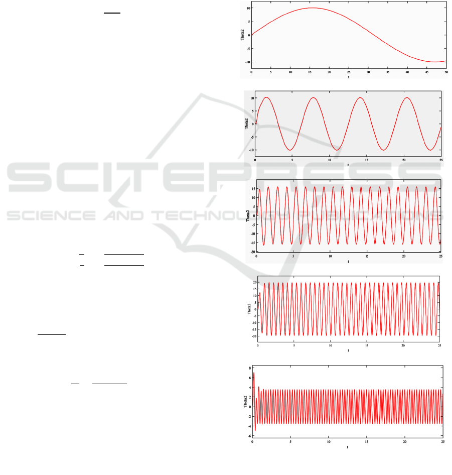
shown in Figure 2 for k=1 and Figure 3 for k=10.
(a)
(b)
(c)
(d)
(e)
Figure 2: Closed loop control response for M=4, N=6 k=1
and ω = (a) 0.1 Hz, (b) 1 Hz, (c) 5 Hz, (d) 10 Hz, (e) 20
rad/sec.
Closed - Loop Control of Plate Temperature using Inverse Problem
423
(a)
(b)
(c)
(d)
(e)
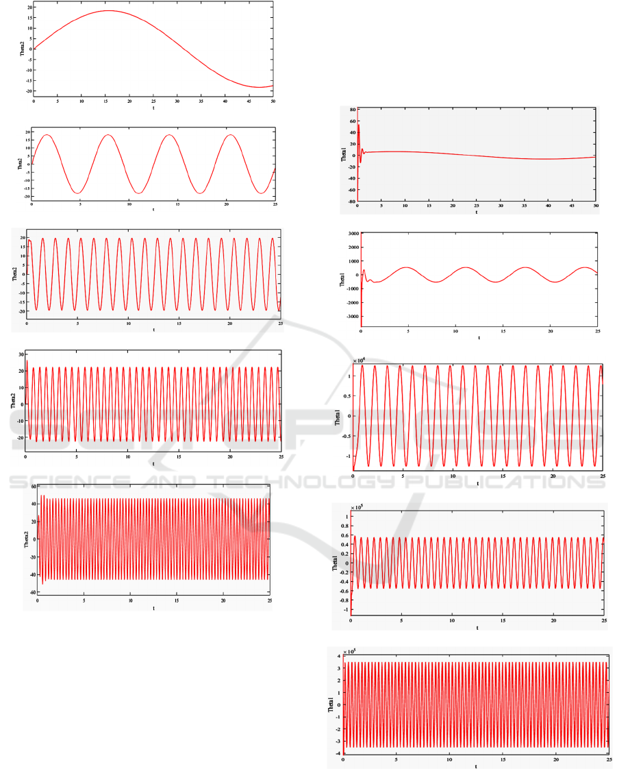
Figure 3: Closed loop control response θ2for M=4, N=6
k=10 and ω = (a) 0.1 Hz, (b) 1 Hz, (c) 5 Hz, (d) 10 Hz, (e)
20 rad/sec.
The simulation results in Figure 2 for k=1 and in
Figure 3for k=10 represent the outputs of the closed
loop control θ
with N=6, M=4 terms for⍵ = 0.1, 1,
5, 10 and 20 rad/sec. The output temperature
results in Figure 2 and 3, for lower frequencies of
0.1 and 1 rad/sec, compared to desired one,
20sin⍵t, are very close. The results for output
temperature θ
, for higher frequencies of 5 and 10
rad/sec, compared to desired one, 20sin⍵t, and of
the command temperature θ
, are significantly
different. This can be explained by the very high
amplitudes of the output of the inverse problem,
shown in Figure 4, which lead eventually to an ill-
posed inverse problem at higher frequencies,
particularly with regard to parameters L and α
uncertainty.
(a)
(b)
(c)
(d)
(e)
Figure 4: Inverse problem response θ
1
for M=4, N=6 k=1
and ω = (a) 0.1 Hz, (b) 1 Hz, (c) 5 Hz, (d) 10 Hz, (e) 20
rad/sec.
ICINCO 2016 - 13th International Conference on Informatics in Control, Automation and Robotics
424
For ⍵ = 20, the amplitude is significantly lower
than in for lower frequencies in Figure 2 (e) and
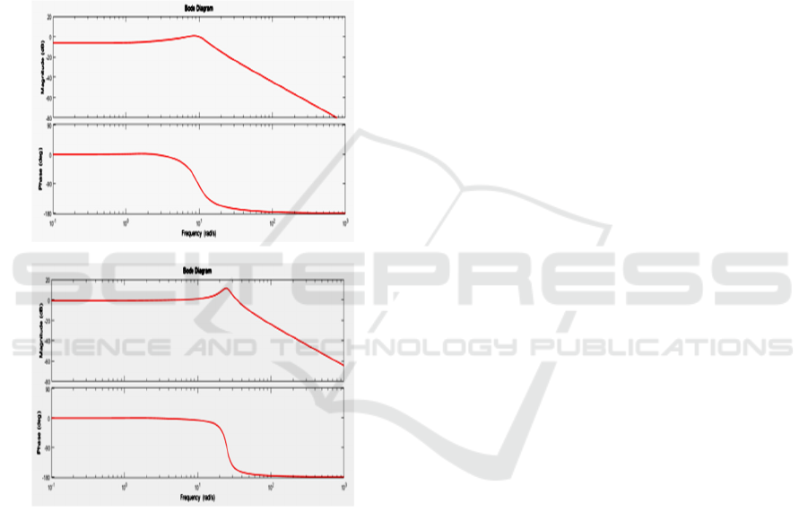
somewhat lower in Figure. 3(e). Bode diagrams of
open loop control transfer function in Figure. 5
explain this by indicating significantly lower
magnitudes for ⍵> 11 rad/sec in Figure 5 (a) for
k=1 and for ⍵>20 rad/sec in Figure 5 (b) for k=10.
In the case of open loop control, since there is no
feedback from the output, parameter uncertainty and
disturbance effects cannot be reduced [9]. Figure 5
shows the Bode diagram of closed loop control
transfer function for N=6 and M=4. and for k=1 in
(a) and k=10 in (b).
(a)
(b)
Figure 5: Bode diagram of closed loop control transfer
function for N=6 and M=4.and (a) k=1and (b) k=10.
4 CONCLUSIONS
The temperature on the one face of a plate can be
controlled in real-time to a desired value from the
other face using the proposed closed loop approach,
based on inverse problem solution. Simulation
results indicate the advantages and the limitations of
this approach. Closed loop control has to be further
investigated to improve the performance and range
of applications to multi-layer plates.
REFERENCES
Beck J. et al., 1985, Inverse Heat Conduction, John
Wiley& Sons.
Fan C. et al., 2009, “A simple method for inverse
estimation of surface temperature distribution on a flat
plate,” Inverse Problems in Science and Engineering,
Vol. 17, No. 7, pp. 885-899.
Feng Z. et al., 2010, “Real-time solution of heat
conduction in a finite slab for inverse analysis,”
International Journal of Thermal Science, vol. 49, pp.
762-768.
Feng Z. et al., 2010, “Temperature and heat flux
estimation from sampled transient sensor
measurements,” International Journal of Thermal
Sciences, vol. 49, pp. 2385-2390.
Feng Z. et al., 2011, “Estimation of front surface
temperature and heat flux of a locally heated plate
from distributed sensor data on the back surface,”
International Journal of Heat and Mass Transfer, vol.
54, pp. 3431-3439.
Maillet D. et al., 2000, Thermal Quadrupoles: Solving the
Heat Equation through Integral Transforms, John
Willey & Sons.
Monde M.,2000, “Analytical method in inverse heat
transfer problem using Laplace transform technique,”
International Journal of Heat and Mass Transfer, vol.
43, pp. 3965-3975.
Necsulescu D., 2009, Advanced Mechatronics: Monitoring
and Control of Spatially Distributed Systems, Word
Scientific.
Necsulescu D., Jarrah B., 2016, Temperature Control of
Thin Plates, CDSR Conf., Ottawa.
Piazzi A., Visioli A., 2001, Robust Set-Point Constrained
Regulation via Dynamic Inversion, Int. Journal of
Robust and Nonlinear Control, 11, pp. 1-22.
Closed - Loop Control of Plate Temperature using Inverse Problem
425
