
Local Point Control of a New Rational Quartic Interpolating Spline
Zhi Liu
1
, Kai Xiao
1
, Xiaoyan Liu
2
and Ping Jiang
1
1
School of Mathematics, Hefei University of Technology, Tunxi Road, Hefei, China
2
Department of Mathematics, University of La Verne, Third Steet, La Verne, U.S.A.
Keywords: Rational Quartic Interpolating Spline, Monotonicity-preserving, C
2
Continuity, Function Value Control,
Derivative Value Control.
Abstract: A new rational quartic interpolating spline based on function values is constructed. The rational quartic
interpolating spline curves have simple and explicit representation with parameters. The monotonicity-
preserving, C
2
continuity and boundedness of rational quartic interpolating spline curves are confirmed.
Function value control and derivative value control of rational quartic interpolation spline are given
respectively. The advantage of these control methods is that they can be applied to modifying the local
shape of interpolating curve only by selecting suitable parameters according to the practical requirements.
1 INTRODUCTION
In engineering and science, one often has a number
of data points, obtained by sampling or
experimentation. It is often required to interpolate
the value and derivatives of that original function. In
the mathematical field of numerical analysis,
interpolation is a method of constructing new
function. The polynomial interpolation methods
include Lagrange interpolation, Newton
interpolation, Hermite interpolation, etc. However,
once the interpolation condition is determined, the
interpolation curve will be fixed uniquely. The
classical Vandermode interpolation does not allows
to control the curve, but it is worthy to say that there
are another methods of controlling the shape. We
know the augmented, generalized interpolation
based on the so-called confluent Vandermonde
matrices (Respondek, 2011; 2013; 2016). They
enable to control the slope and convexity of the
curve in other way.
In order to meet the need of the ever-increasing
modeling complexity and to incorporate
manufacturing requirements, shape control becomes
more and more important as curves and surfaces are
constructed. Given the interpolation condition, how
to control the shape of the curve to meet the
practical application is a very meaningful and urgent
problem.
Spline interpolation is a useful and powerful tool
in CAGD and CAD. Spline methods have been
widely used in geometric modeling. The rational
interpolating splines with shape parameters can
modify curves locally or globally, and it is very
convenient for interaction design in geometric
modeling. Their application in shape control has
attracted a great deal of interest. In recent years,
univariate rational spline interpolations with the
parameters have been receiving more attentions. A
rational cubic spline based on function values is
constructed (Duan et al., 1998), which can be used
to control the position and shape of curve or surface.
Duan and Wang constructed rational cubic
interpolation spline (Duan and Wang, 2005a) and
weighted rational cubic interpolation spline (Duan et
al., 2005b) based on function values. Meanwhile,
convexity-preserving, monotonicity-preserving,
error approximation property and region control
property have been given. The interpolation spline
often is required to satisfy some geometric
characteristics (positivity, monotonity, convexity) of
data points in industrial design. A shape-preserving
rational cubic spline with three parameters has been
developed (Abbas et al., 2012; Zhang et al., 2007),
and the convexity control of interpolating surfaces
had been treated. The region control and convexity
control of rational interpolation curves with
quadratic denominators have been achieved
(Gregory, 1986; Sarfraz, 2000). However, rational
quartic interpolating curves have been ignored due
to the complexity of calculation. With the in-depth
research, Wang and Tan constructed a class of
rational quartic interpolation with linear
denominators (Wang and Tan, 2004), and discussed
Liu, Z., Xiao, K., Liu, X. and Jiang, P.
Local Point Control of a New Rational Quartic Interpolating Spline.
DOI: 10.5220/0005959801650171
In Proceedings of the 6th International Conference on Simulation and Modeling Methodologies, Technologies and Applications (SIMULTECH 2016), pages 165-171
ISBN: 978-989-758-199-1
Copyright
c
2016 by SCITEPRESS – Science and Technology Publications, Lda. All rights reserved
165

monotonicity-preserving,
C
2
continuity and error
approximation property. Duan and Bao proposed the
method of local point control of rational cubic
interpolating spline with linear and quadratic
denominators based on function value respectively
(Bao et al., 2009; Duan et al., 2009; Bao et al.,
2010). The methods of local point control of rational
cubic interpolation spline with linear, quadratic and
cubic denominators respectively were discussed
(Duan et al., 2010; Pan et al., 2013). The above
methods can modify shape of curves at a place
flexible by selecting suitable parameters. Duan and
Bao constructs rational cubic interpolating spline
with difference quotient, but their methods can’t
show the expression of the spline curve or the point
control on the last subinterval (Bao et al., 2009;
Duan et al., 2009).
The rational quartic interpolating spline based on
function values is constructed and studied in this
paper. In section 2, the rational interpolation spline
with parameters based on function values will be
constructed. In this section, monotonicity-
preserving, C
2
continuity and boundedness of
rational quartic interpolating curves are proved. The
method of function value control and derivative
value control of rational quartic interpolation spline
()Pt
will be discussed in section 3. In section 4, for
the end subintervals, point control of rational quartic
interpolation curves
()Pt
are given. Finally, some
examples of local point control methods are shown.
2 RATIONAL QUARTIC
INTERPOLATING SPLINE AND
PROPERTIES
Let
,,0,1,,
ii
tf i n
be a set of given data
points, where
01 n
at t t b ,
and
i
f
is the value of the function being interpolated
at the knot
i
t
. Denote
1ii i
ht t
,
i
i
tt
h
,
1ii
i
i
f
f
h
.
And let
i
be positive parameters, where
0,1, , 1in
. Then C
1
-continuous, piecewise
rational quartic splines with the quadratic
denominator are defined on the interpolating
subinterval
1
,
ii
tt
as follow
1
[, ]
() () (), 0,1, , 1,
ii
ii
tt
Pt pt qt i n
(1)
where
432
2
34
1
() 1 1 1
1,
iiiii
ii
pt f U V
Wf
2
2
() 1
ii
qt
,
and
1
1
11
,1,2,,1,
,0,1,,1,
2,0,1,,2,
iiii
iiii
ii ii
Uffi n
Vff i n
Wf hi n
0
U
and
1n
W
are free variables. It is easy to prove
that the rational quartic spline
()
P
t
satisfies
interpolation condition:
(),0,,
ii
Pt f i n
,
and
() , 1,2, , 1.
ii
Pt i n
Let
() (), 1,2,, 1.
ii
Pt Pt i n
According to the interpolation condition, the
following conclusion can be obtained.
Theorem 1. (C
2
-continuous) When parameters
i
satisfy the equations as follow:
11 1 1iii i ii i i i i
hhhh
,
1, 2, , 1in
, the rational quartic spline (1) keep
C
2
-continuous at interval
0
,
n
tt
.
Specially, consider equidistant knots case, that is
ij
hh
for all
,0,1,,1ij n
. The C
2
-
continuous condition of rational quartic spline can
be simplified as follow:
11
21
ii i i i
.
(2)
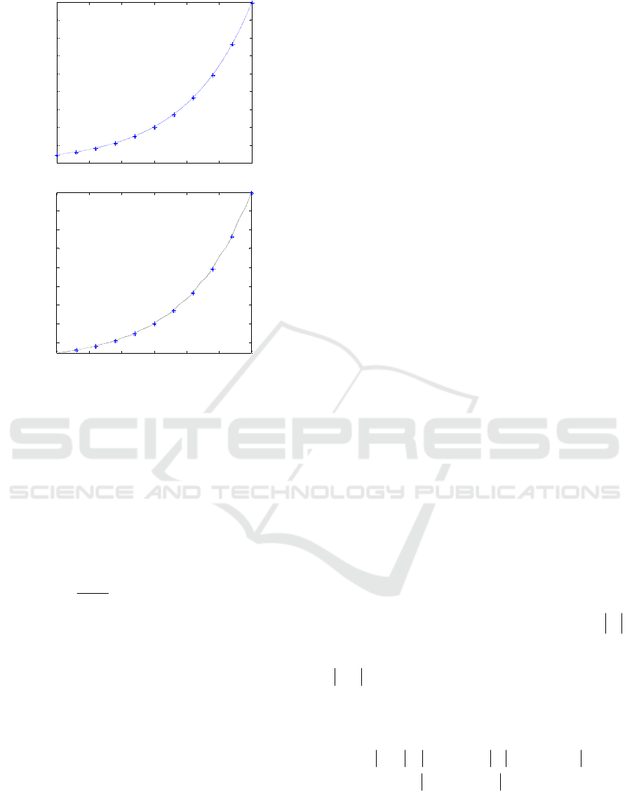
Example 1. Set
() , 1.5,1.5
t
ft e t
as Fig. 1(a). The
C
2
-continuous rational quartic
spline curve
()
P
t
with
0
1
where
1.5
i
tih
,
0,1, ,10i
,
0.3h
,
0
0.5243U
,
9
5.4787W
is given as Fig. 1(b).
SIMULTECH 2016 - 6th International Conference on Simulation and Modeling Methodologies, Technologies and Applications
166
-1.5 -1 -0.5 0 0.5 1 1. 5
0
0.5
1
1.5
2
2.5
3
3.5
4
4.5
(a) The original function.
-1.5 -1 -0.5 0 0.5 1 1.5
0.5
1
1.5
2
2.5
3
3.5
4
(b) The rational quartic interpolation curve.
Figure 1: The C
2
-continuous rational quartic interpolation.
Theorem 2. (Monotonicity-preserving) If the data
points
,,0,1,,
ii
tf i n
satisfy the condition
0
i
, the rational quartic splines (1) satisfy
() 0Pt
when
05/6
i
,
1
/2
ii i
or
5/6 2
i
,
1
/5/3
ii
.
Proof. The
()Pt
can be presented in the simpler
form as
5
5
,
2
0
1
() 1
()
k
k
ik
k
i
Pt Q
qt
(3)
1
,
ii
ttt
,
0,1, , 2in
, where
2
,0
2
,1
,2 1
,3 1
,4 1
,5 1
2
53
3
2
iii
iiiii
iiiii
iiiii
iiii
ii
Q
Q
Q
Q
Q
Q
Obviously, inequality
,
0( 0, ,5)
ik
Qk are true
when
0
i
,
1
/5/3
ii
and
1
/24
ii i
. So,
() 0Pt
when
05/6
i
,
1
/2
ii i
or
5/6 2
i
,
1
/5/3
ii
.
According to the above conclusion, the rational
quartic spline (1) is monotonicity-preserving if and
only if the shape parameters
i
satisfies
0
i
,
05/6
i
,
1
/2
ii i
or
5/6 2
i
,
1
/5/3
ii
.
To make it easier to analyze the properties of the
rational quartic splines, Eq. (1) can be rewritten as
01122
() ( , ) ( , ) ( , )
ii ii ii
P
tff f
(4)
where
43 2
2
0
2
2
32
2
1
2
34 2
2
32
2
(, ) 1 1 1
/1 ,
(, ) 1 1
31 /1 ,
(, ) 1 / 1 .
i
ii
ii
i
ii
(5)
For all
0,1
, the basis function (, )
j
i
satisfy
2
0
(, ) 1
ji
j
.
For the given data, no matter what the parameters
i
might be, the interpolating function defined by (1)
are bounded in the interpolation interval as described
by the following Theorem 3.
Theorem 3. (Boundedness) Given interpolation data
,,0,1,,
ii
tf i n
and all
0
i
, where the
knots are equidistant. Let
()
P
t
be the interpolating
functions defined by (1) and define
2
max
i
j
ji
Nf
.
The values of
()
P
t
in
1
,
ii
tt
satisfy
() 3 /2Pt N
.
Proof. For all
1
,
ii
ttt
,
0,1, , 2in
,
0,1
, it is easy to show that
011
22
() ( , ) ( , )
(, )
ii ii
ii
Pt f f
f
.
According to Eq. (5),
Local Point Control of a New Rational Quartic Interpolating Spline
167

2
23
2
2
0
2
3
2
2
121
(, )
1
21
1
1
12 1
i
ji
j
i
i
thus
() 3 /2Pt N
(6)
So, the proof is completed.
3 LOCAL POINT CONTROL OF
RATIONAL INTERPOLATION
QUARTIC SPLINES
In general, the common spline interpolation is the
fixed interpolation which means the shape of the
interpolating curve or surface is fixed for the given
interpolating data. However, for the quartic rational
interpolation splines defined by Eq (1), although the
interpolation conditions remain unchanged, we can
still adjust the value of shape parameters
i
to
obtain the ideal shape. Thus, function value control
and derivative value control can be carried out at any
point on the quartic rational interpolation curve.
The curve through a fixed point is often
demanded in geometric design. Let
*
be the local
coordinate of a point
*
1
,
ii
ttt
,
1, , 2in
.
The point control of rational quartic interpolation
curve on the end subinterval will be discussed in
section 4.
In the practical design, it is often been required
that the function value of the curve at the point
*
t
to
be equal to a real number
*
M
*
1
ii
f
Mf
. Let
** *
011
*
22
(,) (,)
(,)
ii ii
ii
M
ff
f
(7)
The above equation is called a control equation; it is
equivalent to
0
i
AB
(8)
where
**2
2
*
** *
1
*2 * *2 * * *
12
1
1,
1
11.
i
i
ii
f
A
fM
BffM
If there exist parameters
i
satisfying Eq. (8)
when
,0AB
, there must exist positive
i
satisfying Eq. (7). Therefore, we have the following
function value control theorem.
Theorem 4. Let
()Pt
be interpolation functions
over
1
,
ii
tt
defined in (1), and let
*
1
,
ii
ttt
,
1, , 2in
. The sufficient condition for existence
of positive parameters
i
satisfying
**
()Pt M is
0AB
.
If
**
()Pt M is required, it is equivalent to
0
i
AB
. Thus,
**
()Pt M can set up if and
only if
0, 0AB can’t set up at the same time.
On the other hand, in the practical design, it is
often been required that the first derivative of the
interpolation at the point
1
,
ii
ttt
to be equal to a
real number
M
.
Let
011
22
(, ) (, )
(, )
ii ii
ii
tt
ff
M
f
(9)
Then the control equation (9) is equivalent to
2
012
0
ii
AAA
(10)
where
4
01
112
2
2
1
4
221
12 1 ,
12 24 2 3
212 1,
21 .
iii
ii i
iii
ii i
AffhM
Aff f
hM f f
AffhM
If there exist positive parameters
i
satisfying Eq.
(10), then (9) holds. This can be stated as the
following derivative value control theorem.
Theorem 5. Let
()Pt
be the interpolation function
over
1
,
ii
tt
defined in (1), and let
1
,
ii
ttt
. The
sufficient condition for existence of the positive
parameters
i
satisfying
P
tM
is that Eq. (10)
has positive roots.
Example 2. Without loss of generality, consider the
interpolation on
0,1
. Let
()
f
t
be the interpolated
function satisfying
(0) 1f
,
(1) 2.5f
(2) 4f
and
()
P
t
be interpolation functions defined by (1)
in the interpolating interval
0,1
. It is obvious that
(0)/(10)tt
. The function value control is
shown in Figure 2(a).
SIMULTECH 2016 - 6th International Conference on Simulation and Modeling Methodologies, Technologies and Applications
168
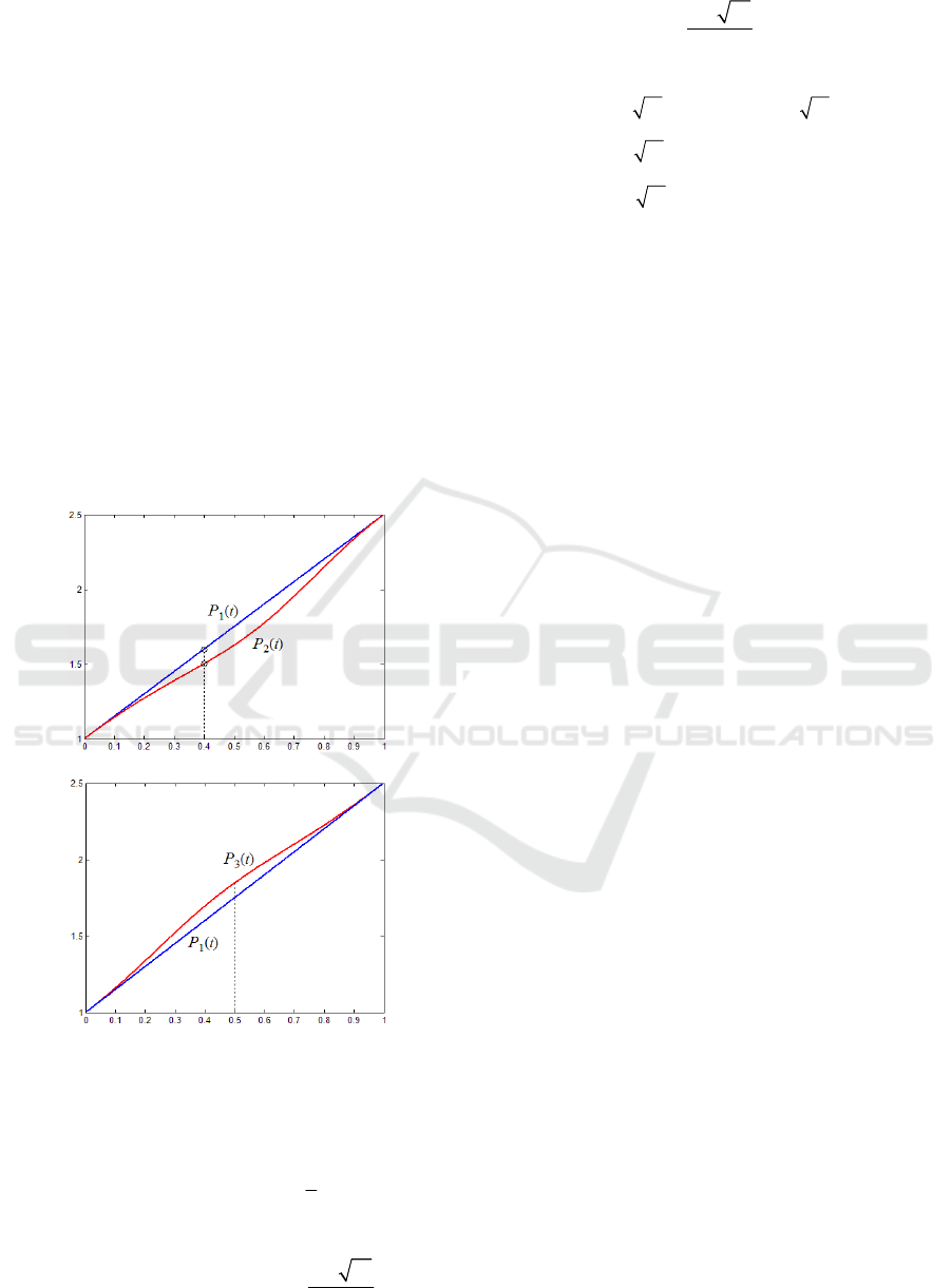
Let
1.5
i
. It can be computed that
(0.4) 1.5383P
. If
(0.4) 1.60P
is required, then
Eq. (8) should be satisfied, and
1
i
which satisfy
Eq. (8). Thus, the interpolation function becomes
4322
1
3422
( ) (1 ) 3.5 (1 ) 3.5 (1 )
3.5 (1 ) 2.5 / (1 )
P
tttttt
tt t tt
,
0,1t
. Furthermore, if
(0.4) 413/ 275 1.5383P
is required,
2
i
can be selected from Eq. (8) and
the interpolation function becomes
4322
2
3422
() 2(1) 7(1) 4.5(1)
3.5 (1 ) 2.5 / 2(1 )
P
tttttt
tt t tt
,
0,1t
.
(a) The function value control.
(b) The derivative value control.
Figure 2: Local point control of rational interpolation
quartic splines.
Example 3. For the same interpolation conditions in
Example 2, let
0.75
i
. It can be calculated that
(0.5) 1.4694P
. Let 0.5t
,
1.40M
in Eq.
(10). It is can be obtained that
2
71670
ii
.
Solving the above equation
815
7
i
can be
obtained. For
815
7
i
, the interpolation
function becomes
43
3
22 3 4
22
() (8 15)(1 ) (28 3.5 15)(1 )
(25.5 15) (1 ) 24.5 (1 ) 17.5
/8 15(1 ) 7 ,
Pt t t t
tt tt t
tt
0,1t
. If
(0.5) 1.50P
is required, according to
Eq. (10), we can obtain the equation
2
210
ii
, calculating that
1
i
, then the
interpolation function becomes
1
()
P
t
. The derivative
value control is shown in Figure 2(b).
4 THE END SUBINTERVAL
POINT CONTROL OF
RATIONAL QUARTIC
INTERPOLATION CURVES
As discussed earlier, the given interval
[,]ab
is
divided into n subintervals
1
[, ]
ii
tt
,
(1,2,,)in
.
Unlike in (Bao et al., 2009), We could construct
()Pt
in every subintervals, including end
subintervals. We use examples to illustrate the point
control of rational interpolation curves
()Pt
.
Without loss of generality, we take
3n . Namely,
there are three subintervals and the curve has three
sections. The general principles are given in
Theorem 4 and 5.
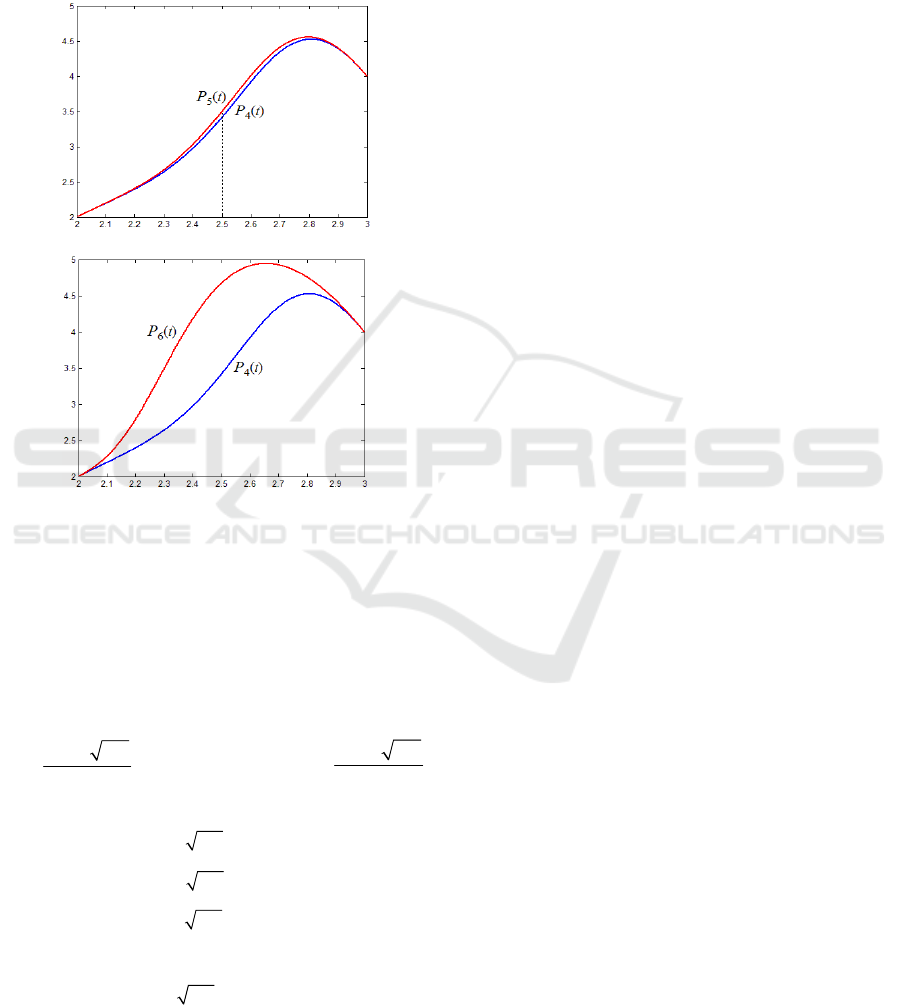
Example 4. Let
()
P
t
be defined by (1),
0
0t
,
1
1t
,
2
2t
,
3
3t
and
0
1f
,
1
3f
,
2
2f
,
3
4f
,
2
13W
, we discuss the function value
control of
()Pt
on the last subinterval,
2,3t
.
The function value control is shown in Figure 3(a).
Let
2
2.0
. The interpolation function is
4322
4
34
22
( ) 4(3 ) 12( 2)(3 ) 8( 2) (3 )
13( 2) (3 ) 4( 2)
/2(3 ) ( 2) ,
P
tttttt
ttt
tt
2,3t
. It can be computed that
4
(2.5) 3.4167P
.
Furthermore, if
4
(2.5) 3.5P
is required, then
2
1.75
can be selected from Theorem 4 and the
interpolation function becomes
Local Point Control of a New Rational Quartic Interpolating Spline
169
4322
5
34
22
( ) 14(3 ) 42( 2)(3 ) 30( 2) (3 )
52( 2) (3 ) 16( 2)
/7(3 ) 4( 2) ,
P
tttttt
ttt
tt
2,3t
.
(a) The function value control.
(b) The derivative value control.
Figure 3: Local point control of rational interpolation
quartic splines on the last subinterval.
Example 5. For Example 4, let
2
2.0
. It can be
computed that
(0.5) 1.4694P
. Let 2.5t , it can
be computed that
(2.5) 7.7778P
. If
(2.5) 8.0P
is required, it can be obtained that
2
22
11 3 0
from Theorem 5. After calculating, we get
2
11 133
7
,
0
i
, we take
2
11 133
7
and the interpolation function becomes
4
6
3
22
34
22
() 22 2 133 (3 )
66 6 133 ( 2)(3 )
14 2 133 ( 2) (3 )
26( 2) (3 ) 8( 2)
/11133(3)2(2),
Pt t
tt
tt
ttt
tt
2,3t
. The function value control is shown in
Figure 3(b).
5 CONCLUSIONS
In this paper, a C
2
rational quartic function has been
developed for the smooth and pleasing visualization
of provided data. It can be testified that rational
quartic interpolation spline is C
2
-continuous,
monotonicity-preserving and bounded. Function
value control and derivative value control of rational
quartic interpolation splines with difference quotient
are given. Rational quartic interpolation splines can
be changed locally by selecting the corresponding
parameters. Thus, they can meet the needs of the
practical design.
ACKNOWLEDGEMENTS
The authors would like to thank the referees for their
valuable comments which greatly help improve the
clarity and quality of the paper.
This work was supported in part by the National
Natural Science Foundation of China (Grant No.
61472466 and 11471093), Key Project of Scientific
Research, Education Department of Anhui Province
of China under Grant No. KJ2014ZD30. The
Fundamental Research Funds for the Central
Universities under Grant No. JZ2015HGXJ0175.
REFERENCES
Abbas, M., Majid, A.A., Ali, J.M. 2012. Monotonicity-
preserving C
2
rational cubic spline for monotone data.
Applied Mathematics and Computation.
Bao, F.X., Sun, Q.H., Duan, Q., 2009. Point control of the
interpolating curve with a rational cubic spline.
Journal of Visual Communication and Image
Representation.
Bao, F.X., Sun, Q.H., Pan, J.X., Duan, Q., 2010. Point
control of rational interpolating curves using
parameters. Mathematical and Computer Modeling.
Duan, Q., Djidjeli, K., Price, W.G., Twizell, E.H., 1998. A
rational cubic spline based on function values.
Computers & Graphics.
Duan, Q., Wang, L.Q., 2005a. A new weighted rational
cubic interpolation and its approximation. Applied
Mathematics and Computation.
Duan, Q., Wang, L.Q., Twizell, E.H., 2005b. A new C
2
based on function values and constrained control of
the interpolating curves. Applied Mathematics and
Computation.
Duan, Q., Bao, F.X., Du, S.T., Twizell, E.H., 2009. Local
control of interpolating rational cubic spline curves.
Computer-Aided Design.
Duan, Q., Liu, X.P., Bao, F.X., 2010. Local shape control
of the rational interpolation curves with quadratic
SIMULTECH 2016 - 6th International Conference on Simulation and Modeling Methodologies, Technologies and Applications
170

denominator. International Journal of Computer
Mathematics.
Gregory, J.A., 1986. Shape preserving spline interpolation,
Computer-Aided Design.
Pan, J.X., Sun, Q.H., Bao, F.X., 2013. Shape control of the
curves using rational cubic spline. Journal of
Computational Information Systems.
Respondek, J.S., 2016. Incremental numerical recipes for
the high efficient inversion of the confluent
Vandermonde matrices. Computers and Mathematics
with Applications.
Respondek, J.S., 2011. Numerical recipes for the high
efficient inverse of the confluent Vandermonde
matrices. Applied Mathematics and Computation.
Respondek, J.S., 2013. Recursive numerical recipes for the
high efficient inverse of the confluent Vandermonde
matrices, Applied Mathematics and Computation.
Sarfraz, M., 2000. A rational cubic spline for the
visualization of monotonic data, Computers &
Graphic.
Wang, Q., Tan, J.Q., 2004. Rational quartic spline
involving shape parameters. Journal of information
and Computational Science.
Zhang, Y.F., Duan, Q., Twizell, E.H., 2007. Convexity
control of a bivariate rational interpolating spine
surfaces, Computers & Graphics.
Local Point Control of a New Rational Quartic Interpolating Spline
171
