Joint Integrated Track Splitting for Multi-sensor Multi-target Tracking

in Clutter

Yifan Xie

, Haeho Lee

, Myonghwan Ahn

, Bum Jik Lee

and Taek Lyul Song

Department of Electronic Systems Engineering, Hanyang University, Ansan, Republic of Korea

Combat System R&D Lab, LIG Nex1 Co. Ltd., Seongnam, Republic of Korea

Submarine Combat System Part, Daewoo Shipbuilding & Marine Engineering, Seoul, Republic of Korea

Keywords:

Multitarget, Multisensor, Target Existence, Joint Integrated Track Splitting, S-D Assignment.

Abstract:

Automatic object tracking for track initialization, conﬁrmation and termination can be realized by using the

probability of target existence, which is a track quality measure for false track discrimination. In this paper,

we present a multi-sensor multi-target tracking application based on the probability of target existence and

multi-sensor joint integrated track splitting (MS-JITS), which is an extension of JITS framework to multi-

sensor systems. For fair comparison, incorporation of the target existence paradigm and the S-D assignment

is implemented. This work also consummates the S-D assignment based estimators for track management by

the probability of target existence.

1 INTRODUCTION

In many target tracking surveillance systems, such

as air trafﬁc control or ground target tracking for

multiple targets, measurements can be received from

multiple sensors. Because of the limited sensing re-

gion of sensors, a single sensor can only partially

access information of the environment. Information

from multiple sensors can be combined using data

fusion algorithms to achieve cooperative observation

effects (Xiong and Svensson, 2002). However the

target tracker has no prior knowledge on the origin

of each measurement, which terms multi-dimensional

assignment (MDA) problem (Gilbertand and Hofstra,

1988) in multi-sensor systems. Pattipatti et al. pro-

posed the S-D assignment algorithm to solve this non-

deterministic polynomial-time hard (NP-hard) prob-

lem. By using the Lagrangian(dual) relaxation ap-

proach, the problem is then solved as a series of 2-D

subproblems (Pattipati et al., 1992; Deb et al., 1997).

In multi-target scenario, a mechanism is required

to decide the source (clutter or particular track) of

received measurements, and the objective is to as-

sociate measurement-to-track. This problem turns

more critical in multi-sensor multi-target situations,

where the sensor fusion problem has to be overcomed

as well. The conventional solutions for multi-target

tracking (MTT) include joint probabilistic data as-

sociation (JPDA) (Blackman and Popoli, 1999) and

multi-hypothesis tracking (MHT)(Reid, 1979; Black-

man, 2004), etc. For multi-sensor scenarios, multi-

sensor JPDA (Frei and Pao, 1998; Pao and Frei, 1995)

and multi-sensor MHT (Kirubarajan et al., 2001) are

proposed. These algorithms enumerate all possible

measurement to target allocations, and use likelihood

to evaluate each hypothesis. The number of hypothe-

ses grows exponentially in the number of tracks and

the number of measurements involved. The computa-

tional cost in generating the possibilities to data as-

sociation is usually excessive when the number of

tracks and number of measurements are large. There-

fore, suboptimal solutions with computational feasi-

bility are required.

Integrated track splitting (ITS) (Mu

sicki et al.,

2007; Shi et al., 2015b) is a suboptimal multi-scan

single target estimator, that is capable of false track

discrimination (FTD) using the probability of target

existence as a track quality measure. The false track

discrimination identiﬁes the true tracks and eliminates

false alarms, which is of the essential functionality

in track maintenance (Song et al., 2013; Song et al.,

2015c; Song et al., 2015a). The probability of target

existence for false track discrimination is obtained by

a simple equation which utilizes the parameters in-

volved in the associate probability calculations. ITS

has been extended for dealing with multi-target as

joint integrated track splitting (JITS) (Mu

sicki and

Xie, Y., Lee, H., Ahn, M., Lee, B. and Song, T.

Joint Integrated Track Splitting for Multi-sensor Multi-target Tracking in Clutter.

DOI: 10.5220/0005960102990307

In Proceedings of the 13th International Conference on Informatics in Control, Automation and Robotics (ICINCO 2016) - Volume 1, pages 299-307

ISBN: 978-989-758-198-4

299

Evans, 2009; Shi et al., 2015a). Similar to MHT, each

component of JITS forms the history of measurement

hypotheses involved in the track for multiple scans.

The JITS algorithm is also able to distinguish between

the true tracks and false alarms by recursively calcu-

lating the probability of target existence.

In this paper, we present a sub-optimal multi-

sensor multi-scan multi-target tracking algorithm

based on the JITS algorithm, which we call multi-

sensor joint integrated track splitting (MS-JITS). A

comparison between the S-D assignment algorithm

and the MS-JITS algorithm is also conducted.

Problem formulation is detailed in Section II. Sec-

tion III presents the general MS-JITS algorithm. An

application of target existence paradigm to S-D as-

signment is described in Section IV. A simulation

study which demonstrates the performance of MS-

JITS is given in Section V, followed by the concluding

remarks in Section VI.

2 PROBLEM FORMULATION

2.1 Measurement Model

A number of measurements of sensors are received at

each sampling time k synchronously. Due to the un-

certainty of measurement origins, the received mea-

surements may originate from the target or clutter. Let

denote the target detection probability of sensor s.

Since the targets are not always detectable, P

< 1.

The gating process selects measurements from

sensor s and forms a validated measurement set y

(k)

with cardinality m

at time k, y

s,i

(k) indicates the ith

element of y

(k). P

is the probability that the true

measurement falls in the gate if target exists. Denote

= {y

(k),Y

k−1

} as the set of validated measure-

ments up to time k. And a collection of all sensor

measurement is Y

= {Y

,...,Y

2.2 Target Model

The target dynamics are modeled in Cartesian coor-

dinates. Under the additive noise assumption, the τth

target kinematic and measurement equations for track

τ at k scan are deﬁned by

= F

k−1

+ ω

, (1)

s,k

= H

+ v

s,k

. (2)

where x

is the target τ state vector, z

s,k

is the tar-

get measurement. F

and H

are the transition matrix

and measurement matrix of sensor s respectively. The

process noise ω

and measurement noise v

s,k

are as-

sumed to be zero-mean, uncorrelated white Gaussian

noise sequences with known covariance Q

and R

s,k

As for track existence state, ψ

is the event that

target τ exists. On the contrary,

suggests that target

τ does not exist at scan k.

2.3 Clutter Model

The number of clutter measurements in the surveil-

lance space follows Poisson distribution. The clut-

ter measurement density at point y

s,i

(k) is denoted

by ρ

s,i

(k) , ρ(y

s,i

(k)). Spatial distribution of clutter

measurements is assumed to be uniform in the surveil-

lance space.

3 MS-JITS ALGORITHM

3.1 Single-sensor JITS

3.1.1 Track State

The track state probability density function (pdf) con-

ditioned on the measurement set Y

at time k is given

p(x

,ψ

) = p(x

|ψ

)P(ψ

), (3)

where P(ψ

) represents the probability of target

existence of track τ. It also suggests that the track

state pdf is always calculated conditioned on the tar-

get existence event ψ

. Speciﬁcally, the track state

pdf is approximated by a Gaussian mixture of mutu-

ally exclusive and exhaustive track components such

p(x

|ψ

) =

∑

|ψ

)p(x

,ψ

). (4)

The track component c

consists of the following

compositions:

• given measurement history;

• trajectory state pdf p(x

,ψ

);

• component probability ξ

|ψ

), which is in-

dexed by c

, subjects to the constraint of

∑

|ψ

) = 1. (5)

3.1.2 Track Prediction

Track state predicted pdf involved in propagating

from time k − 1 to k yields

p(x

,ψ

k−1

) = p(x

|ψ

k−1

)P(ψ

k−1

). (6)

ICINCO 2016 - 13th International Conference on Informatics in Control, Automation and Robotics

300

Assumed that the target is always observable when-

ever it exists, then the existence and observability can

be modeled with Markov Chain 1 (Mu

sicki et al.,

1994). The predicted target existence is given by

P(ψ

k−1

) = ∆

1,1

P(ψ

k−1

), (7)

where ∆

1,1

is the Markov transition probability.

The predicted track state pdf is denoted as

p(x

|ψ

k−1

) =

∑

k−1

|ψ

k−1

) ×

p(x

k−1

,ψ

k−1

). (8)

Relative track component probabilities do not change

during the propagation. Each track component prop-

agates individually based on the prediction step of the

Kalman ﬁlter such that yields

p(x

k−1

,ψ

k−1

) = N(x

; ˆx

k|k−1

k−1

k|k−1

k−1

)). (9)

3.1.3 Measurement Selection

Each track component selects measurements from

sensor s separately, the validated measurements will

be included in the set y

(k). And the relevant mea-

surement likelihood becomes

k,i

k−1

) , p(y

s,i

(k)| ˆx

k|k−1

k−1

))

N(y

s,i

(k); H ˆx

k|k−1

k−1

)),

(10)

where

k−1

) is predicted measurement error co-

variance. The mixed likelihood for the common mea-

surement shared by components in track τ becomes

k,i

∑

k−1

k,i

k−1

). (11)

3.1.4 Joint Multi-target Data Association

In order to reduce the computational complexity,

tracks that share common validated measurements are

termed a cluster. Joint multi-target data association is

performed simultaneously for each cluster.

A joint event ε is an assignment among possible

assignments of all measurements to all tracks in the

cluster, and it must obey the principle that each track

is assigned with zero or one measurement; each mea-

surement is assigned to zero or one track. The joint

events are mutually exclusive (Mu

sicki and Evans,

2009).

Set T

(ε) is composed by tracks with no allocated

measurement; Set T

(ε) is the collection of tracks al-

located one measurement; i(ε, τ) indicates that mea-

surement i in ε is allocated to track τ. And the corre-

sponding joint event probability is

P(ε|Y

) = C

−1

∏

ε∈T

(ε)

[1 − P

P(ψ

k−1

)] ×

∏

ε∈T

(ε)

P(ψ

k−1

)

(i(ε,τ))

s,i

(k)

], (12)

where C

is the normalization constant, p

(i(ε,τ)) is

the likelihood that measurement i originates from tar-

get τ. Since the joint events are mutually exclusive,

they form an exhaustive set

∑

P(ε|Y

) = 1. (13)

A set of all joint events that measurement i is as-

signed to track τ is denoted by Ξ(i, τ). Hypothesis

(i) denotes that measurement i is the detection of

target τ at time k, and the probability of θ

(i) satisﬁes

p(θ

(0)|Y

) =

∑

ε∈Ξ(0,τ)

P(ε|Y

), (14)

p(ψ

,θ

(0)|Y

) =

(1 − P

)P(ψ

k−1

)

1 − P

P(ψ

k−1

)

p(θ

(0)|Y

) (15)

p(ψ

,θ

(i)|Y

) =

∑

ε∈Ξ(i,τ)

P(ε|Y

). (16)

The data association probabilities based on the as-

sumption of target existence are then given by

k,i

, p(θ

(i)|ψ

)

p(ψ

,θ

(i)|Y

)

P(ψ

)

. (17)

3.1.5 Track Update

The track state pdf is updated by the measurements in

(k). The update track state can be obtained from the

Bayes rule

p(x

,ψ

) = p(x

|ψ

)P(ψ

) (18)

where the posterior probability of target existence is

given by

P(ψ

) =

∑

i=0

p(ψ

,θ

(i)|Y

) (19)

The track state a posterior pdf p(x

|ψ

) is a mix-

ture of all track components pdf such that

p(x

|ψ

) =

∑

|ψ

)p(x

,ψ

) (20)

Joint Integrated Track Splitting for Multi-sensor Multi-target Tracking in Clutter

301

where track component posterior probability

|ψ

) is given by

|ψ

) =

(

k−1

|ψ

k−1

)β

k,i

,i = 0

k−1

|ψ

k−1

)β

k,i

k−1

)

k,i

,i 6= 0

(21)

where i = 0 represents the hypothesis that none of the

validated measurements originate from the target.

Then updated by using Kalman ﬁlter with mea-

surement y

s,i

(k),

p(x

,ψ

) = N(x

; ˆx

k|k

)), (22)

[ ˆx

k|k

)] = KF

s,i

(k), ˆx

k|k−1

k−1

k|k−1

k−1

),H

s,k

], (23)

where the KF

stands for the Kalman ﬁlter update.

3.1.6 Component Management

Without component control, the number of track com-

ponents increase exponentially in time, thus efﬁcient

management is crucial. The component management

in JITS involves two parts: merging and pruning.

Component merging deals with track components

with similar features, for which we applied a rela-

tively short retained track component history as sim-

ilarity measure. Component pruning is to remove

those track components with low probability, so that

track is always composed by more signiﬁcant compo-

nents (Challa et al., 2011).

3.2 Multi-sensor JITS

Figure 1: Sequential implementation of JITS algorithm.

Difﬁculties for generalizing a single sensor JITS ﬁl-

ter to a multi-sensor case are complicated. Since the

sensors are synchronized and the measurement noises

across the sensors are uncorrelated, the two update

schemes are available: parallel processing and se-

quential update. In the parallel processing, the sen-

sor measurements are transmitted to a fusion center

and converted with respect to a reference coordinate

system. The target state is updated by applying the

JITS algorithm to the measurements in the fusion cen-

ter. However, it requires a solution for multiple de-

tection target tracking as the measurements contain

multiple detections of a target gathered from differ-

ent sensors(Habtemariam et al., 2013). To realize the

parallel processing, sensors need to be synchronized

and heavy data trafﬁc to the fusion center is expected.

The rigorous formulas are too complicated for practi-

cal usage (Smith and Singh, 2006)(Bar-Shalom et al.,

2011).

In the sequential update, the target state is up-

dated with the data from one sensor at a time. The

essence of sequential update for multi-sensor JITS al-

gorithm is operating single sensor JITS algorithm it-

eratively, so that the computational complexity is sig-

niﬁcantly decreased. Sensors do not have to be syn-

chronized. In (Pao and Frei, 1995), it suggests that

the sequential update gives superior tracking perfor-

mance than the parallel process when data association

is considered. This is primarily due to fact that better

ﬁltered estimates are available after processing each

sensor’s data. Measurement selection procedure ﬁl-

ters out many measurements that are not statistically

signiﬁcant. And as a consequence, the sequential up-

date scheme, which is computationally tractable and

with better tracking performance, is applied for solv-

ing multi-sensor problem in this paper.

The way of implementing the sequential update

for the MS-JITS algorithm is to process the measure-

ments from each sensor in succession (Bar-Shalom

and Li, 1995), using single-sensor JITS algorithm as

shown in Figure 1. The outputs of the sth (s ≤ S − 1)

sensor are regarded as intermediate track stated pdf of

target τ, state vector ˆx

τ,s

and the covariance

τ,s

. Us-

ing intermediate result in place of the predicted state,

then proceed to the next sensor for updating, and ﬁ-

nally cumulates the ultimate results ˆx

and

in the

last sensor.

[ ˆx

τ,s

k|k

τ,s

k|k

] = JIT S[ ˆx

τ,s−1

k|k

τ,s−1

k|k

(k)],

s = 1, 2, ...S − 1 (24)

[ ˆx

k|k

] = JIT S[ ˆx

τ,s−1

k|k

τ,s−1

k|k

(k)],s = S (25)

where JIT S denotes the single-sensor JITS algorithm

described in Section III-A.

The posterior probability of target existence in

multi-sensor target tracking application should give

due consideration to validated measurements in every

sensor. And it can be calculated by updating target

existence probability iteratively using the joint multi-

target data association method (19) described in Sec-

tion III.

ICINCO 2016 - 13th International Conference on Informatics in Control, Automation and Robotics

302

4 TARGET EXISTENCE

PROBABILITY IN S-D

ASSIGNMENT

Unlike the S-D assignment, all the tracks in MS-JITS

algorithm are automatically managed (conﬁrmation

or termination) by probability of target existence. For

a fair result comparison, it stands to reason that this

method should be applied to S-D assignment.

Every element (including dummy measurement)

in a composite measurement contributes to the poste-

rior probability of target existence. We use the mea-

surement from the ﬁrst sensor to derive an interme-

diate probability of target existence, using it in place

of the predicted probability for the next sensor. The

posterior probability of target existence is given by

P(ψ

) =

(

∏

s=1

)P(ψ

k−1

)

1 − (1 −

∏

s=1

)P(ψ

k−1

)

, (26)

where Λ

is the measurement likelihood ratio in sen-

sor s, denoted by

(

1 − P

+ P

k,i

s,i

(k)

if κ

s,i

= 1

1 − P

otherwise

. (27)

The binary variable κ

s,i

= 1 indicates that y

s,i

(k) is the

measurement of target τ. The measurement likelihood

k,i

(indexed by sensor s) is given by

k,i

(

N(y

s,i

(k); ˆx

k|k−1

),s = 1

N(y

s,i

(k); ˆx

τ,s−1

k|k

),s = 2, 3, ..., S

(28)

where S

is the predicted measurement covariance of

the standard Kalman ﬁlter. The posterior probability

of target existence is given in (26), for the sake of

brevity, the superscript τ is omitted for Λ

, p

k,i

. The

derivation is described in appendix.

5 SIMULATION

This section provides a comparison between the MS-

JITS algorithm and the S-D assignment algorithm

(S = 3) by simulating the scenarios with varying clut-

ter measurement densities and target detection proba-

bilities respectively.

Three targets are observed in clutter on a two di-

mensional surveillance region with 1000 m in length

and 400 m in width. The clutter measurements are as-

sumed to be uniformly distributed. Figure 2 shows a

representative trial over the entire Monte Carlo trials.

The illustrated arrows and crosses are the trajectories

for each target and clutter measurements respectively.

Figure 2: Surveillance region.

The selection window size is given with gating

probability P

= 0.99. The measurements noise is as-

sumed to be Gaussian distributed with zero-mean and

standard deviation σ

= 5m. The target state vector

consists of

= [x,y, ˙x, ˙y]

(29)

with transition matrix F







1 0 T 0

0 1 0 T

0 0 1 0

0 0 0 1







. (30)

The velocity vectors of the targets are

[13m/s,−6.25m/s]

,[15m/s,0m/s]

,[13m/s,6.25m/s]

respectively. Sampling time is T = 1s. Target maxi-

mum velocity is v

max

= 25m/s. The process noise is

zero-mean with covariance

= q







0 T







, (31)

where q = 0.75 m

Tracks are initialized automatically using two-

point differencing (Challa et al., 2011), and a constant

value of probability of target existence is assigned to

each newly initialized track. The probability of target

existence is recursively updated in subsequent scans.

If the probability exceeds the conﬁrmation threshold,

the corresponding track is conﬁrmed. And the track

will be terminated if the probability falls below the

termination threshold. The Markov transitional prob-

ability is 4

1,1

= 0.98.

Three scenarios of this experiment are consid-

ered, each with a different target detection probabil-

ity and clutter measurement density: A. clutter mea-

surement density ρ

s,i

(k) = 1 × 10

−4

and low target

detection probability P

= 0.6; B. clutter measure-

ment density ρ

s,i

(k) = 2 × 10

−4

and high target de-

tection probability P

= 0.9; C. clutter measurement

Joint Integrated Track Splitting for Multi-sensor Multi-target Tracking in Clutter

303

density ρ

s,i

(k) = 2 × 10

−4

and low target detection

probability P

= 0.6. The Monte Carlo simulations

for each scenario consist of 200 trails. MS-JITS is

updated by a Gaussian mixture of component state

pdf such that most of the measurements in the val-

idation window contributes to the update. The esti-

mator based on S-D assignment chooses the compos-

ite measurement by evaluating maximum likelihood

and the global nearest neighbor using 2-D dynamic

assignment algorithm (Popp et al., 2001).

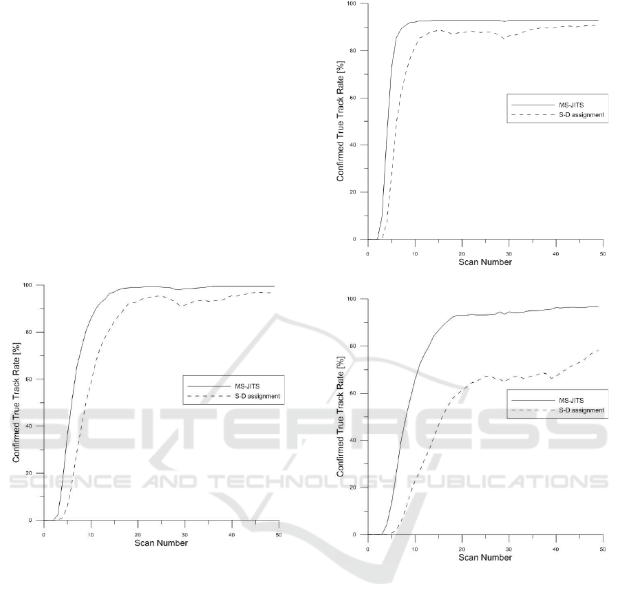
5.1 False Track Discrimination

The false track discrimination results are shown in

Figures 3, 4 and 5. The graphs show the percentage

of conﬁrmed true tracks of MS-JITS and S-D assign-

ment over time for each scenario.

Figure 3: Conﬁrmed true track rate-Scenario A.

MS-JITS always conﬁrms track faster than S-D

assignment. These ﬁgures show that MS-JITS has

superior advantage of true track conﬁrmation, which

is apparent in dense clutter density and low detection

probability environment.

In the simulation, the false alarm rates of the MS-

JITS algorithm of the 3 scenarios are 3.3%, 0.86%,

2.5% compared with the S-D assignment algorithm

of 25%, 11.67%, 32.5%. The inequality of the re-

sult is due to the fact that the essences of each algo-

rithm are distinct. In the target state update part, the

MS-JITS algorithm processes all the validated mea-

surement, whereas the S-D assignment algorithm pro-

cesses only one composite measurement that marginal

target information is utilized. If efforts were made to

minimize the gap of false alarm rates, the time dura-

tion that conﬁrmation procedure required would de-

crease and the total conﬁrmed true track rate would

Figure 4: Conﬁrmed true track rate-Scenario B.

Figure 5: Conﬁrmed true track rate-Scenario C.

increase for the MS-JITS algorithm.

5.2 Retention Test

Retention test is designed for observing the destina-

tion of every conﬁrmed true track. Then we can eval-

uate the efﬁciency of an algorithm. The following in-

formation is obtained by tagging the conﬁrmed true

tracks at scan 15 and checking them again at scan 40

(Mu

sicki, 2006):

• nCases: Total number of tracks that following a

target at scan 15;

• nOK: Total number of tracks that still following

the original target at scan 40;

• nLost: Total number of tracks that not following

any target at scan 40;

ICINCO 2016 - 13th International Conference on Informatics in Control, Automation and Robotics

304

• nSwitched: Total number of tracks that end up fol-

lowing a different target at scan 40;

• nMerged: Total number of tracks disappeared due

to merging between scan 15 and 40.

The target retention tests are listed in Table 1-3.

Table 1: Retention Statistics-Scenario A.

MS-JITS S-D

nCases 583 509

nOK 559 392

nLost 5 42

nSwitched 16 72

nMerged 3 3

Table 2: Retention Statistics-Scenario B.

MS-JITS S-D

nCases 561 541

nOK 544 377

nLost 1 85

nSwitched 16 70

nMerged 0 9

Table 3: Retention Statistics-Scenario C

MS-JITS S-D

nCases 520 279

nOK 481 137

nLost 11 99

nSwitched 23 42

nMerged 5 1

The results show that track retention capabilities

of MS-JITS, with success rates (nOK / nCases) of

96%, 97%, 93%, is better than S-D assignment, with

success rates of 77%, 70%, 49%. The percentage of

false alarms is apparently decreased. In addition, the

nLost and nSwitched number is much reduced in MS-

JITS. That displays the track trajectory maintains well

during propagation.

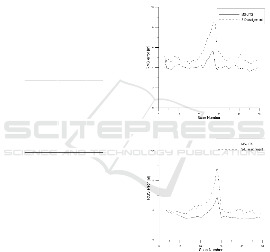
5.3 RMS error

Position root mean square (RMS) error is a criterion

for evaluating track trajectory accuracy, and for sim-

plicity each scenario shows the representative result

only. The results are presented in Figures 6, 7 and

8, which show the RMS errors of MS-JITS and S-

D assignment for different scenarios. The salients in

every ﬁgure are shown around scan 25, which is the

time that the close encounter between the tracks oc-

curred. Due to the incorrect measurement-to-track

association, some measurements are allocated to the

unrelated track. Therefore, the track trajectory esti-

mation accuracy degenerates. Obviously, MS-JITS

always provides better trajectory estimate than S-D

assignment.

Figure 6: RMS error in position-Scenario A.

Figure 7: RMS error in position-Scenario B.

5.4 Computation Time

The computation time of both algorithms for each

scenario are listed in Table 4.

It suggests that the MS-JITS algorithm requires

more computation time, which provides a trade off

between the computation time and tracking perfor-

Joint Integrated Track Splitting for Multi-sensor Multi-target Tracking in Clutter

305

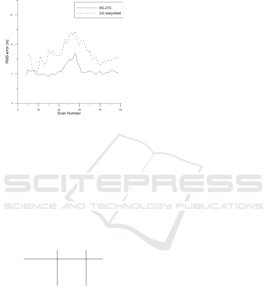
Figure 8: RMS error in position-Scenario C.

mance in practical applications. Though the com-

putational load of MS-JITS is heavier, for some sit-

uations where track trajectories are located in near

vicinity, MS-JITS is more preferable. A compro-

mise of the computation time and estimation accuracy

can be achieved by adopting an iterative implemen-

tation (Song et al., 2015b) for the JITS ﬁlter. The

computational requirements and estimation accuracy

can be classiﬁed into several levels by adjusting the

number of iterations. The iterations start with single

target tracking algorithm and each subsequent itera-

tion improves the approximation towards the optimal

multi-target solution within a ﬁnite number of itera-

tions. The application of iterative JITS ﬁlter for multi-

sensor system remains further exploration.

Table 4: Computation Time (sec.).

MS-JITS S-D

Scenario A 262 82

Scenario B 6691 415

Scenario C 4063 456

6 CONCLUSIONS

In this paper, we have presented a JITS based multi-

sensor tracking algorithm, which is capable of false

track discrimination by using the probability of target

existence as a track quality measure. And the S-D as-

signment based estimator is enhanced by incorporat-

ing the probability of target existence for false track

discrimination.

The S-D assignment algorithm may be effective in

applications where computational efﬁciency is more

important. But in situations where clutter measure-

ment density is dense or target detection probability

is low, the composite measurements become seriously

contaminated or mostly consisted by dummy mea-

surements. And as a consequence, the false alarm rate

rises and track trajectory accuracy decreases. In con-

trast, the MS-JITS algorithm compensates the draw-

backs at the cost of computational load. The MS-JITS

algorithm processes measurement information more

comprehensively with a more strict mechanism to dis-

tinguish the true tracks and false alarms. In addition,

the retention test proves that the MS-JITS algorithm

has stronger robustness. Thus, for applications where

track trajectory accuracy and track maintenance are

preferable, the MS-JITS algorithm offers an attractive

alternative.

ACKNOWLEDGEMENTS

This paper was supported by the LIG-Nex1 Co., Ltd.

under the contract LIGNEX1-2015-0108(00).

REFERENCES

Bar-Shalom, Y. and Li, X. (1995). Multitarget-multisensor

tracking: principles and techniques. YBS Publishing.

Bar-Shalom, Y., Willett, P. K., and Tian, X. (2011). Track-

ing and Data Fusion. YBS Publishing.

Blackman, S. (2004). Multiple hypothesis tracking for mul-

tiple target tracking. IEEE Aerospace and Electronic

Systems Magazine, 19(1):5–18.

Blackman, S. and Popoli, R. (1999). Design and Analysis

of Modern Tracking Systems. Artech House.

Challa, S., Morelande, M. R., Mu

sicki, D., and Evans, R. J.

(2011). Fundamentals of object tracking. Cambridge

University Press.

Deb, S., Yeddanapudi, M., Pattipati, K., and Bar-Shalom,

Y. (1997). A generalized s-d assignment algorithm

for multisensor-multitarget state estimation. IEEE

Transactions on Aerospace and Electronic Systems,

33(2):523–538.

Frei, C. W. and Pao, L. Y. (1998). Alternatives to monte-

carlo simulation evaluations of two multisensor fusion

algorithms. Automatica, 34(1):103–110.

Gilbertand, K. C. and Hofstra, R. B. (1988). Multidi-

mensional assignment problems. Decision Sciences,

19(2):306–321.

Habtemariam, B., Tharmarasa, R., Thayaparan, T., Mallick,

M., and Kirubarajan, T. (2013). A multiple-detection

joint probabilistic data association ﬁlter. IEEE Jour-

nal of Selected Topics in Signal Processing, 7(3):461–

471.

ICINCO 2016 - 13th International Conference on Informatics in Control, Automation and Robotics

306

Kirubarajan, T., Wang, H., Bar-Shalom, Y., and Pattipati,

K. R. (2001). Efﬁcient multisensor fusion using mul-

tidimensional data association. IEEE Transactions on

Aerospace and Electronic Systems, 37(2):386–400.

sicki, D. (2006). Track score and target existence. In 9th

Int. Conf. on Information Fusion, pages 1–7.

sicki, D., Evans, R., and Stankovi

c, S. (1994). Integrated

Probabilistic Data Association (IPDA). IEEE Trans.

Automatic Control, 39(6):1237–1241.

sicki, D. and Evans, R. J. (2009). Multiscan multitarget

tracking in clutter with integrated track splitting ﬁlter.

IEEE Transactions on Aerospace and Electronic Sys-

tems, 45(4):1432–1447.

sicki, D., Scala, B. F., and Evans, R. J. (2007). The in-

tegrated track splitting ﬁlter efﬁcient multi-scan sin-

gle target tracking in clutter. IEEE Transactions on

Aerospace and Electronic Systems, 43(4):1409–1425.

Pao, L. Y. and Frei, C. W. (1995). A comparison of parallel

and sequential implementations of a multisensor mul-

titarget tracking algorithm. In American Control Con-

ference, Proceedings, volume 3, pages 1683–1687.

Pattipati, K. R., Deb, S., Bar-Shalom, Y., and Washburn,

R. B. (1992). A new relaxation algorithm and pas-

sive sensor data association. IEEE Transactions on

Aerospace and Electronic Systems, 37(2):198–213.

Popp, R. L., Pattipati, K. R., and Bar-Shalom, Y. (2001).

m-best s-d assignment algorithm with application to

multitarget tracking. IEEE Transactions on Aerospace

and Electronic Systems, 37(1):22–39.

Reid, D. (1979). An algorithm for tracking multiple targets.

IEEE Transactions Automatic Control, 24(6):843–

854.

Shi, Y. F., Song, T. L., and Lee, J. H. (2015a). Multi-

target tracking in clutter using a high pulse repetition

frequency radar. IET, Radar, Sonar and Navigation,

9(8):1047–1054.

Shi, Y. F., Song, T. L., and Mu

scki, D. (2015b). Tar-

get tracking in clutter using a high pulse repetition

frequency radar. IET, Radar, Sonar and Navigation,

9(3):299–307.

Smith, D. and Singh, S. (2006). Approaches to multisen-

sor data fusion in target tracking: a survey. IEEE

Transactions on Knowledge and Data Engineering,

18(12):1696–1710.

Song, T. L., Kim, H., and Mu

sicki, D. (2015a). Dis-

tributed (nonlinear) target tracking in clutter. IEEE

Transactions on Aerospace and Electronic Systems,

51(1):654–668.

Song, T. L., Kim, H. W., and Musicki, D. (2015b). Itera-

tive joint integrated probabilistic data association for

multitarget tracking. IEEE Transactions on Aerospace

and Electronic Systems, 51(1):642–653.

Song, T. L., Mu

scki, D., and Kim, Y. (2015c). Multitarget

tracking with state dependent detection. IET, Radar,

Sonar and Navigation, 9(1):10–18.

Song, T. L., Mu

sicki, D., Kim, H. W., and Govaers, F.

(2013). Gaussian mixture tracking: Mht and its com-

parison. In Sensor Data Fusion: Trends, Solutions,

Applications (SDF), pages 1–6.

Xiong, N. and Svensson, P. (2002). Multi-sensor manage-

ment for information fusion: issues and approaches.

In 5th Int. Conf. on Information Fusion, volume 3,

pages 163–186.

APPENDIX

Sequential Likelihood Ratio

This section is used to describe the posterior proba-

bility of target existence in MS-JITS algorithm. The

measurements from the ﬁrst sensor are used to com-

pute an intermediate posterior probability of target ex-

istence P(ψ

τ,1

), with corresponding measurement

likelihood ratio Λ

denoted by

P(ψ

τ,1

) =

P(ψ

k−1

)

1 − (1 − Λ

)P(ψ

k−1

)

. (32)

After gating the measurements in next sensor, tar-

get existence probability is updated,

P(ψ

τ,2

) =

P(ψ

τ,1

k−1

)

1 − (1 − Λ

)P(ψ

τ,1

k−1

)

. (33)

Substituting the P(ψ

τ,1

k−1

) by equation (32) yields,

P(ψ

τ,2

) =

P(ψ

k−1

)

1−(1−Λ

)P(ψ

k−1

)

1 − (1 − Λ

)

P(ψ

k−1

)

1−(1−Λ

)P(ψ

k−1

)

P(ψ

k−1

)

1 − (1 − Λ

)P(ψ

k−1

)

. (34)

Similarly, we can obtain

P(ψ

τ,3

) =

P(ψ

k−1

)

1 − (1 − Λ

)P(ψ

k−1

)

. (35)

Finally, up to sensor S yields

P(ψ

) =

(

∏

s=1

)P(ψ

k−1

)

1 − (1 −

∏

s=1

)P(ψ

k−1

)

. (36)

Joint Integrated Track Splitting for Multi-sensor Multi-target Tracking in Clutter

307