
Experimental Results of Trajectory Tracking Control of Robot
Manipulator using Time Varying Sliding Mode Controller
Yasuhiko Mutoh and Nao Kogure
Department of Engineering and Applied Sciences, Sophia University, 7-1 Kioicho, Chiyoda-ku, Tokyo, Japan
Keywords:
Sliding Mode Control, Time-varying Pole Placement Control, Trajectory Tracking Control, Nonlinear System,
Linear Time Varying System.
Abstract:
The author et al. proposed the design method of the sliding mode controller for the trajectory tracking control
problem of nonlinear systems. This controller consists of the conventional sliding mode control and the pole
placement controller for the the linear time varying approximate model of the nonlinear system around the
desired trajectory. In this paper, this controller is applied to the trajectory tracking control of the actual 2-link
robot manipulator, and, experimental results are shown.
1 INTRODUCTION
The pole placement control for linear time varying
systems is argued in (Nguyen,1987)(Val´aˇsek,1995).
The author et al. proposed the simple design
method of the pole placement controller for linear
time varying systems using the concept of the rela-
tive degree of the system (Mutoh,2011) (Mutoh and
Kimura,2011). Using this controller, a time varying
closed loop system becomes equivalent to some lin-
ear time invariant system that has desired constant
eigenvalues, by the state feedback. This implies that
if we apply the pole placement controller to a linear
time varying system, any control technique for linear
time invariant systems can be applied to the equiva-
lent time invariant closed loop system.
From this point of view, the authors (Mutoh and
Kogure,2014) proposed to make use of this technique
for designing the sliding mode controller for linear
time varying systems and this controller was applied
to the trajectory tracking control of nonlinear sys-
tems. The nonlinear system has a linear time vary-
ing approximate model around some desired trajec-
tory. The design procedure is as follow. The first step
is to find the pole placement state feedback for the
linear time varying approximate system, by which the
closed loop system is equivalent to some linear time-
invariant system. Then, by using the conventional
sliding mode control technique, the sliding mode con-
trol input for this linear time invariant system can be
obtained (Utkin,1992). Finally, using an equivalent
time varying transformation matrix, this control in-
put can be transformed into the sliding mode control
for the original linear time varying system. By this
controller, the linear time varying approximate model
around the desired trajectory ia stabilized, which im-
plies the trajectory tracking controller for this nonlin-
ear system is obtained.
In this paper, this type of controller is applied to
the actual 2-link robot manipulator, and, the experi-
mental results are shown. Here, both of continuous
and discrete sliding mode controllers are used. In
the following, the pole placement controller for lin-
ear time varying systems and a continuous and dis-
crete types of the sliding mode controllers are sum-
marized in Section 2 and 3, respectively. Then, Sec-
tion 4 presents how these controllers are used for the
trajectory tracking control of nonlinear systems. And,
finally, some experimental results are shown in Sec-
tion 5.
2 POLE PLACEMENT FOR
LINEAR TIME VARYING
SYSTEMS
2.1 Controllability of Linear Time
Varying Systems
Consider the following linear time-varying multi-
input system.
˙x(t) = A(t)x(t) + B(t)u(t) (1)
Mutoh, Y. and Kogure, N.
Experimental Results of Trajectory Tracking Control of Robot Manipulator using Time Varying Sliding Mode Controller.
DOI: 10.5220/0005961304390446
In Proceedings of the 13th International Conference on Informatics in Control, Automation and Robotics (ICINCO 2016) - Volume 1, pages 439-446
ISBN: 978-989-758-198-4
Copyright
c
2016 by SCITEPRESS – Science and Technology Publications, Lda. All rights reserved
439

Here, x(t) ∈ R
n
and u(t) ∈ R
m
are the state variable
and the input signal, respectively. A(t) ∈ R
n×n
and
B(t) ∈ R
n×m
are time varying coefficient matrices,
which are bounded and smooth functions of t.
The matrix B(t) is written as follows, using its col-
umn vectors b
i
(t) ∈ R
n
(i = 1, ··· , m).
B(t) =
b
1
(t) b
2
(t) ··· b
m
(t)
(2)
Let b
i
k
(t) ∈ R
n
be defined by the following recur-
sive equations.
b
0
k
(t) = b
k
(t)
b
i
k
(t) = A(t)b
i−1
k
(t) −
˙
b
i−1
k
(t)
(3)
k = 1, 2···m, i = 1, 2· ··
Then, the controllability matrix of the system (1) is
defined as follows.
U
c
= [b
0
1
(t)··· b
0
m
(t)|··· |b
n−1
1
(t)··· b
n−1
m
(t)] (4)
Theorem 1. The system (1) is completely control-
lable if and only if
rankU
c
(t) = n
∀
t (5)
If the system (1) is completely controllable, the
controllability indices, µ
1
, µ
2
,···, µ
m
, can be defined,
and
m
∑
i=1
µ
i
= n. (6)
Using these controllability indices, the following non-
singular matrix, R(t), can be defined.
R(t) =
h
b
0
1
(t)·· · b
µ
1
−1
1
(t)|·· · |b
0
m
(t)·· · b
µ
m
−1
m
(t)
i
(7)
In this paper, it is assumed that the system is com-
pletely controllable, and, its controllability indices
satisfy the inequality, µ
1
≥ µ
2
≥ ··· ≥ µ
m
, without loss
of generality.
2.2 Time Varying Pole Placement
Control
The problem of pole placement control for the time-
varying system (1) is to find the state feedback so that
the time-varying closed loop system is equivalent to
some time-invariant system which has desired con-
stant eigenvalues.
Suppose that the system (1) is completely
controllable and has the controllability indices,
µ
1
, µ
2
, ··· , µ
m
. Let
˜
C(t) ∈ R
m×n
be defined by
˜
C(t) = W(t)R
−1
(t) (8)
where
W(t) = diag(w
1
(t), w
2
(t), ··· , w
m
(t))
w
i
(t) = [0, ··· , 0, λ
i
(t)] ∈ R
1×µ
i
(i = 1, · ·· , m)
(9)
λ
i
(t) 6= 0.
Using
˜
C(t), a new output signal ˜y(t) is defined as fol-
lows.
˜y(t) =
˜
C(t)x(t) (10)
Then, the vector relative degree from u(t) to ˜y(t) be-
comes (µ
1
, µ
2
, ··· , µ
m
) (Mutoh and Kimura,2011).
Let ˜y(t) and
˜
C(t) be defined by
˜y(t) =
˜y
1
(t)
.
.
.
˜y
m
(t)
,
˜
C(t) =
˜c
1
(t)
.
.
.
˜c
m
(t)
(11)
where, ˜y
i
(t) ∈ R
1
and ˜c
i
(t) ∈ R
1×n
.
From this, the pole placement state feedback is
obtained in the following procedure. Let α
i
j
be the
coefficients of a desired stable polynomial of the dif-
ferential operator p.
α
i
(p) = p
µ
i
+ α
i
µ
i
−1
p
µ
i
−1
+ · ··+ α
i
0
(12)
(i = 1, ··· , m)
Since, the vector relative degree from u(t) to ˜y(t) is
µ
1
, µ
2
, ···, µ
m
, there exist a matrix D(t) ∈ R
m×n
and
a nonsingular matrix Λ(t) ∈ R
m×m
satisfying the fol-
lowing equation.
α
1
(p)
.
.
.
α
m
(p)
˜y(t) = D(t)x(t) + Λ(t)u(t)
(13)
Actually, D(t) and Λ(t) are given by
D(t) =
D
1
(t)
D
2
(t)
.
.
.
D
m
(t)
, Λ(t) =
Λ
1
(t)
Λ
2
(t)
.
.
.
Λ
m
(t)
(14)
and
D
i
(t) = [α
i
0
, α
i
1
, ···α
i
µ
i
−1
, 1]
˜c
0
i
(t)
˜c
1
i
(t)
.
.
.
˜c
µ
i
i
(t)
(15)
Λ
i
(t) = [0, ·· · , 0, λ
i
(t), γ
i(i+1)
(t), ·· · , γ
ij
(t)]
where ˜c
k
i
(t) ∈ R
1×n
and γ
ij
(t) ∈ R
1
are defined as fol-
lows.
˜c
0
i
(t) = ˜c
i
(t)
˜c
j+1
i
(t) = ˜c
j
i
(t)A(t) +
˙
˜c
j
i
(t)
(16)
i = 1, 2··· m, j = 1, 2·· ·
ICINCO 2016 - 13th International Conference on Informatics in Control, Automation and Robotics
440

γ
ij
(t) = c
µ
i
−1
i
(t)b
j
(t) (17)
j = i+ 1, ·· · , m
Thus, by the state feedback
u(t) = −Λ
−1
(t)D(t)x(t) (18)
the closed loop system becomes
α
1
(p)
.
.
.
α
m
(p)
˜y(t) = 0. (19)
This system has the following state realization,
˙
ω(t) = A
∗
ω(t) =
A
∗
1
0
.
.
.
0 A
∗
m
ω(t) (20)
where
A
∗
i
=
0 1 0
.
.
.
.
.
.
.
.
.
.
.
. 1
−α
i
0
. .. . . . −α
i
µ
i
−1
(i = 1, . . . , m) (21)
and,
det(sI − A
∗
) = α
1
(s) · α
2
(s)· ··α
m
(s). (22)
Here, ω(t) ∈ R
n
is a new state vector, and is defined
by
ω(t) =
˜y
1
(t)
.
.
.
˜y
(µ
1
−1)
1
(t)
.
.
.
˜y
m
(t)
.
.
.
˜y
(µ
m
−1)
m
(t)
. (23)
This implies that ω(t) and the original state variable
x(t) satisfy the relation
ω(t) = T(t)x(t) (24)
where
T(t) =
˜c
0
1
(t)
.
.
.
˜c
µ
1
−1
1
(t)
.
.
.
˜c
0
m
(t)
.
.
.
˜c
µ
m
−1
m
(t)
. (25)
Hence, the closed loop system is equivalent to the
time invariant linear system which has the desired
closed loop poles, i.e.,
T(t)(A(t) − B(t)Λ
−1
(t)D(t))T
−1
(t)
−T(t)
˙
T
−1
(t) = A
∗
(26)
The non-singularity of T(t) is guaranteed by the con-
trollability of the system (1).
Note that T(t) is Lyapunov transformation if it is
non-singular and both of T(t) and T
−1
(t) are con-
tinuous and bounded for all t. It is well known
that the exponential stability is preserved between
two equivalent linear time-varying systems if the
transformation matrix is Lyapunov transformation
(Rugh,1993)(Chen,1999). Then, to guarantee the sta-
bility of the closed loop system, T(t) should be the
Lyapunov transformation.
From the above, the pole placement procedure is
summarized as follows.
STEP 1 Using the controllability matrix, U
c
(t),
check the controllability of the system (1) and find
the controllability indices µ
i
(i = 1, ··· , m).
STEP 2 Calculate
˜
C(t) using (8).
STEP 3 From
˜
C(t), calculate ˜c
k
i
(t) and γ
ij
(t) using
(16) and (17).
STEP 4 Determine the coefficients, α
i
j
of desired
closed loop characteristic polynomials in (12).
STEP 5 Using (14) and (15) with the parameters ob-
tained in the above STEP 3 and 4, the pole place-
ment state feedback is given in (18).
3 SLIDING MODE CONTROLLER
DESIGN
3.1 Continuous Sliding Mode Control
In this section, the sliding mode controller design for
the linear time varying system (1) is summarized. In
the previous section, for the given time varying sys-
tem (1), we design the pole placement state feedback
(18). Here, the new input signal v(t) is added to it,
then the pole place ment state feedback becomes as
follows.
u(t) = Λ
−1
(t)(−D(t)x(t) + v(t)) (27)
Hence, the closed loop system,
˙x(t) = (A(t) − B(t)Λ
−1
(t)D(t))x(t) + B(t)v(t) (28)
becomes equivalent to
˙
ω(t) =
A
∗
1
0
.
.
.
0 A
∗
m
ω(t) + B
∗
v(t) (29)
Experimental Results of Trajectory Tracking Control of Robot Manipulator using Time Varying Sliding Mode Controller
441

where
B
∗
= diag[b
∗
1
, b
∗
2
, · ·· , b
∗
m
]
b
∗
i
=
0
.
.
.
0
1
∈ R
µ
i
, i = 1, ··· , m (30)
and the transformation matrix T(t) between x(t) and
ω(t) are defined by (24), (25).
To design the sliding mode controller for the time
varying system (28), we first design the conventional
sliding mode control input v(t) for the equivalent lin-
ear time invariant system (29), and then, transform
v(t) into the sliding mode control input for the system
(28), using the relation (24)(25).
ω(t) and v(t) can be written as follows.
ω(t) =
ω
1
(t)
.
.
.
ω
m
(t)
, v(t) =
v
1
(t)
.
.
.
v
m
(t)
(31)
ω
i
(t) ∈ R
µ
i
, v
i
(t) ∈ R
1
(i = 1, ··· , m)
Then, the system (29) is presented as the set of the
following m subsystems.
˙
ω
i
(t) = A
∗
i
ω
i
(t) + b
∗
i
v
i
(t), (i = 1, ··· , m) (32)
Here, A
∗
i
is defined by (21). As well known, the con-
ventional sliding mode controller for i-the subsystem
is obtained as follows.
First, let the desired stable characteristic polyno-
mial of the i-th sliding dynamics be chosen as follows.
s
i
(p) = p
µ
i
−1
+ s
i
µ
i
−2
p
µ
i
−2
+ · ··+ s
i
0
(33)
Then, the i-th stable sliding surface is given by the
following hyper surface,
S
T
i
ω
i
(t) = [s
i
0
, · ·· , s
i
µ
i
−2
, 1 ]ω
i
(t) = 0. (34)
And, it is also well known that the i-th sliding con-
trol input v
i
(t) which makes the state variable move
toward the sliding surface can be obtained by
v
i
(t) = −(S
T
i
b
∗
i
)
−1
{S
T
i
A
∗
i
ω
i
(t) + q
i
sgn(σ
i
) + k
i
f
i
(σ
i
)}
= −{ S
T
i
A
∗
i
ω
i
(t) + q
i
sgn(σ
i
) + k
i
f
i
(σ
i
)} (35)
where
σ
i
= S
T
i
ω
i
(t) (36)
and q
i
> 0 and k
i
> 0 are constant parameters and
f
i
(σ
i
) is a function such that σ
i
f
i
(σ
i
) > 0. In fact, it is
readily shown that, using (35), we have the following
Lyapunov function.
V =
1
2
m
∑
i=1
σ
2
i
> 0,
˙
V =
m
∑
i=1
σ
i
˙
σ
i
< 0 (37)
Hence, from the above, the pole placement and the
sliding mode control input u(t) for the original system
(1) becomes as follows, using the original state vari-
able x(t).
u(t) = Λ
−1
(t)(−D(t)x(t) + v(t)) (38)
Here, the i-th element of v(t) is
v
i
(t) = −{S
T
i
A
∗
i
T
i
(t)x(t) + q
i
sgn(σ
i
) + k
i
f
i
(σ
i
)}
(39)
and
σ
i
= S
T
i
T
i
(t)x(t) (i = 1, ··· , m) (40)
where from (24)(25),
T
i
(t) =
˜c
0
i
(t)
.
.
.
˜c
µ
i
−1
i
(t)
. (41)
3.2 Discrete Sliding Mode Control
In general, the continuous sliding mode controller has
a chatteringproblem. On the other hand, there is a dis-
crete type of sliding mode controller, which can avoid
the chattering problem. In this paper, we also apply
this type of discrete sliding mode controller from the
practical point of view.
Suppose that the following is a discretized system
of i-th subsystem (i = 1, ·, m)), (32), with the sampling
period, T
s
.
ω
i
(T
s
(k+1)) = F
∗
i
ω
i
(T
s
k)+g
∗
i
v
i
(T
s
k), (i= 1, ·· · , m)
(42)
Here, F
∗
i
and g
∗
i
have the following forms.
F
∗
i
=
0 1 0
.
.
.
.
.
.
.
.
.
.
.
. 1
−β
i
0
. .. . . . −β
i
µ
i
−1
∈ R
µ
i
×µ
i
g
∗
i
=
0
.
.
.
0
1
∈ R
µ
i
, (i = 1, ··· , m) (43)
As the continuouscase, let the desired discrete sta-
ble characteristic polynomial of the i-th sliding dy-
namics be chosen as follows.
ξ
i
(z) = z
µ
i
−1
+ ξ
i
µ
i
−2
z
µ
i
−2
+ · ··+ ξ
i
0
(44)
Here, z is the forward shift operator. Then, the i-th
stable sliding surface is given by the following high-
per surface,
S
T
i
ω
i
(T
s
k) = [ ξ
i
0
, · ·· , ξ
i
µ
i
−2
, 1 ]ω
i
(T
s
k) = 0. (45)
ICINCO 2016 - 13th International Conference on Informatics in Control, Automation and Robotics
442
And, it is also known that the i-th sliding control input
v
i
(T
s
k) which makes the state variable move toward
the sliding surface can be obtained as
v
i
(T
s
k) = −S
T
i
(F
∗
i
− I)ω(T
s
k) − η
i
σ
i
(T
s
k) (46)
where
σ
i
(T
s
k) = S
T
i
ω
i
(T
s
k). (47)
and
0 ≤ η
i
≤ 2. (48)
Further more, if 0 ≤ η
i
≤ 1, the state variable ap-
proaches the sliding surface without chattering, and,
if 1 ≤ η
i
≤ 2, with chattering.
From the above, the pole placement and the dis-
crete sliding mode control input u(t) for the origi-
nal system (1) becomes as follows, using the original
state variable x(t).
u(t) = Λ
−1
(t)(−D(t)x(t) + Zoh[v(T
s
k)])
( T
s
k ≤ t ≤ T
s
(k+ 1) ) (49)
here the i-th element of v(T
s
k) is
v
i
(T
s
k) = −S
T
i
(F
∗
i
− I)ω(T
s
k) − η
i
σ
i
(T
s
k) (50)
and
σ
i
= S
T
i
T
i
(T
s
k)x(T
s
k) (i = 1, ··· , m) (51)
where from (24)(25),
T
i
(T
s
k) =
˜c
0
i
(T
s
k)
.
.
.
˜c
µ
i
−1
i
(T
s
k)
. (52)
Here, Zoh[·] is the zero-order hold.
4 TRAJECTORY TRACKING
CONTROL OF NONLINEAR
SYSTEMS
Consider the following non-linear system.
˙x(t) = f(x(t), u(t)) (53)
Here, x(t) ∈ R
n
and u(t) ∈ R
m
are the state variable
and the input signal. Let x
∗
(t) and u
∗
(t) be some de-
sired trajectory and the desired input for x
∗
(t).
The problem is to design a controller to track this
desired trajectory x
∗
(t) stably around it. This can be
done by stabilizing this trajectory in the neighborhood
of x
∗
(t) and u
∗
(t). Let ∆x(t) and ∆u(t) be defined by
∆x(t) = x(t) − x
∗
(t)
∆u(t) = u(t) − u
∗
(t).
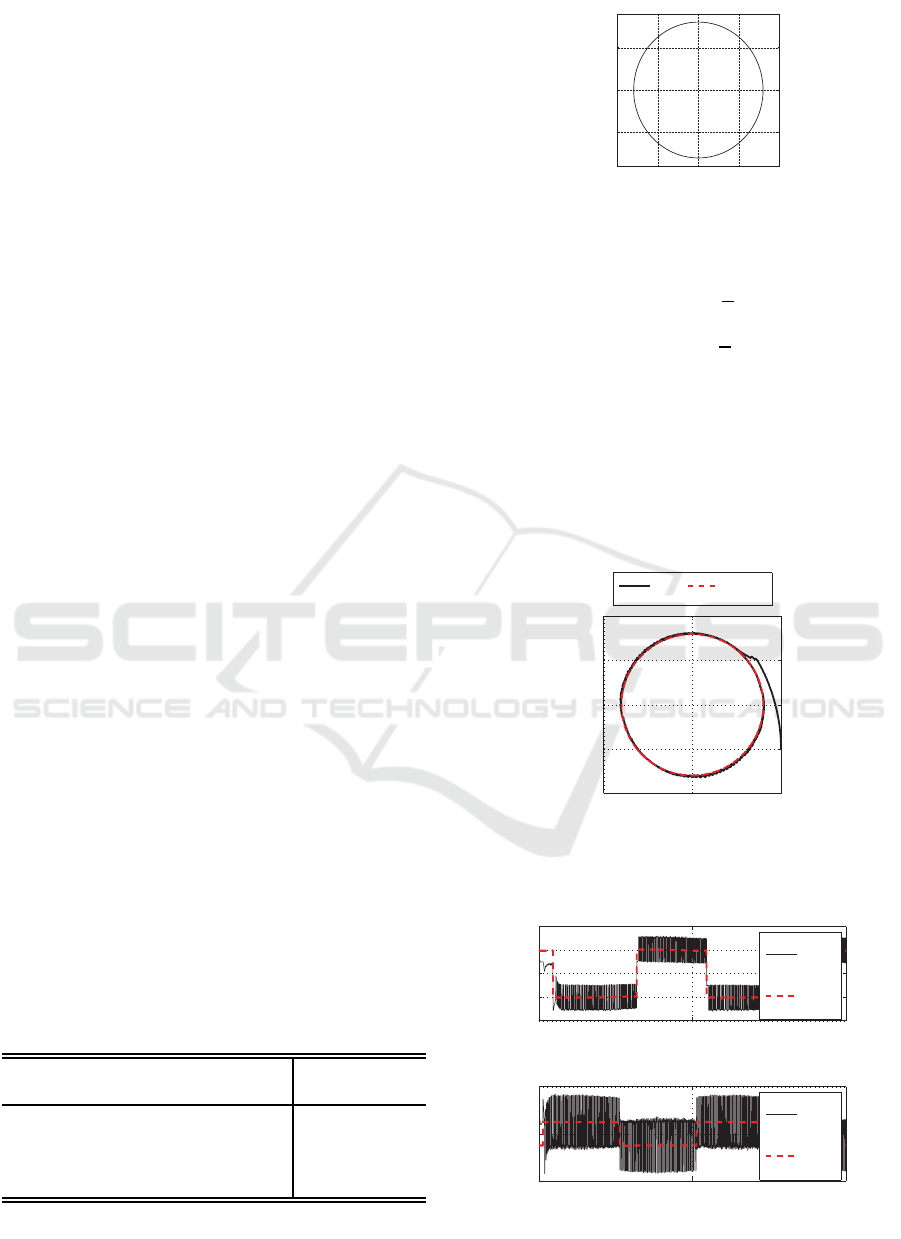
Figure 1: Two-Link Manipulator(SR-402DDII).
Figure 2: A Model of the 2-Link Manipulator.
Then, we have a linear time-varying approximate
model around x
∗
(t) and u
∗
(t) as follows.
∆˙x(t) = A(t)∆x(t) + B(t)∆u(t) (54)
A(t) =
∂
∂x
f(x
∗
(t), u
∗
(t))
B(t) =
∂
∂u
f(x
∗
(t), u
∗
(t))
(55)
Then, using time-varying sliding mode control tech-
nique, error equation can be stabilized around the de-
sired trajectory x
∗
(t) and u
∗
(t). For this purpose, the
time varying pole placement control is first applied
to this linear time varying approximate system. By
which, the closed system is equivalent to some linear
time invariant system. Next, verious types of sliding
mode controllers are applied to this time invariantsys-
tem to obtain the robustness against disturbance.
5 EXPERIMENTAL RESULTS
In this Section, the time varying sliding control tech-
nique was applied to the trajectory tracking problem
of the actual 2-link robot manipulator, and some ex-
perimental results are shown.
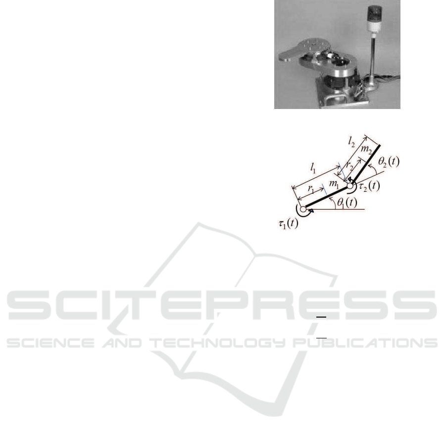
The manipulator used for the experiment is shown
in Fig.1 and its model is depicted in Fig.2. The motion
equation of the manipulator is described as follows.
M(θ(t))
¨
θ(t) +C(θ(t),
˙
θ(t))
˙
θ(t) + D(
˙
θ(t)) = τ(t) (56)
Experimental Results of Trajectory Tracking Control of Robot Manipulator using Time Varying Sliding Mode Controller
443
where,
θ(t) =
θ
1
(t)
θ
2
(t)
M(θ(t)) =
J
1
+ J
2
+ 2m
2
r
2
l
1
cosθ
2
(t),
J
2
+ m
2
r
2
l
1
cosθ
2
(t),
J
2
+ m
2
r
2
l
1
cosθ
2
(t)
J
2
C(θ(t),
˙
θ(t)) =
−2m
2
r
2
l
1
˙
θ
2
(t)sinθ
2
(t),
m
2
r
2
l
1
˙
θ
1
(t)sinθ
2
(t),
−m
2
r
2
l
1
˙
θ(t)
2
sinθ
2
(t)
0
D(
˙
θ(t)) =
2sgn(
˙
θ
1
(t))
0.25sgn(
˙
θ
2
(t))
J
i
= J
l
i
+ m
i
r
2
i
(i = 1, 2). (57)
Here, θ
i
(t) and τ
i
(t) are a joint angle and an input
torque of i-th joint, l
i
and r
i
are a length of the i-th
link and the distance between the i-th joint and the
center of gravity of i-th link, and J
l
i
is the moment of
inertia of i-th link about its center of gravity. D(
˙
θ(t))
is a friction term.
Define a state variablex(t) and an input vector u(t)
by
x(t) =
θ(t)
˙
θ(t)
∈ R
4
, u(t) =
τ
1
(t)
τ
2
(t)
∈ R
2
then, the system, (55), can be rewritten as the follow-
ing state equation.
˙x(t) = f(x(t), u(t))
=
0 I
0 Γ(x(t))
x(t) +
0
Φ(x(t))
u(t)
(58)
where
Γ(x(t)) = −M(θ(t))
−1
C(θ(t),
˙
θ(t)) ∈ R
2×2
Φ(x(t)) = M(θ(t))
−1
∈ R
2×2
. (59)
I ∈ R
2×2
is the identity matrix. The values of physical
parameters of this system are shown in Table 1.
Table 1: Parameters of the Robot Manipulator.
variable link1 link2
(i = 1, 2)
i = 1 i = 2
Mass[kg] m
i
3.43 1.55
Length[m] l
i
0.2 0.2
Center of Gravity[m] r
i
0.1 0.1
Inertia[kgm
2
] J
l
i
0.208 0.03
The desired trajectory of the end portion of the
manipulator is given by the following equation, which
;
>P@
<
>P@
Figure 3: The Desired Trajectory of the End Portion.
is shown in Fig.3
X
∗
= 0.08cos
π
5
t + 0.3 (60)
Y
∗
= 0.08sin
π
5
t + 0.05 (61)
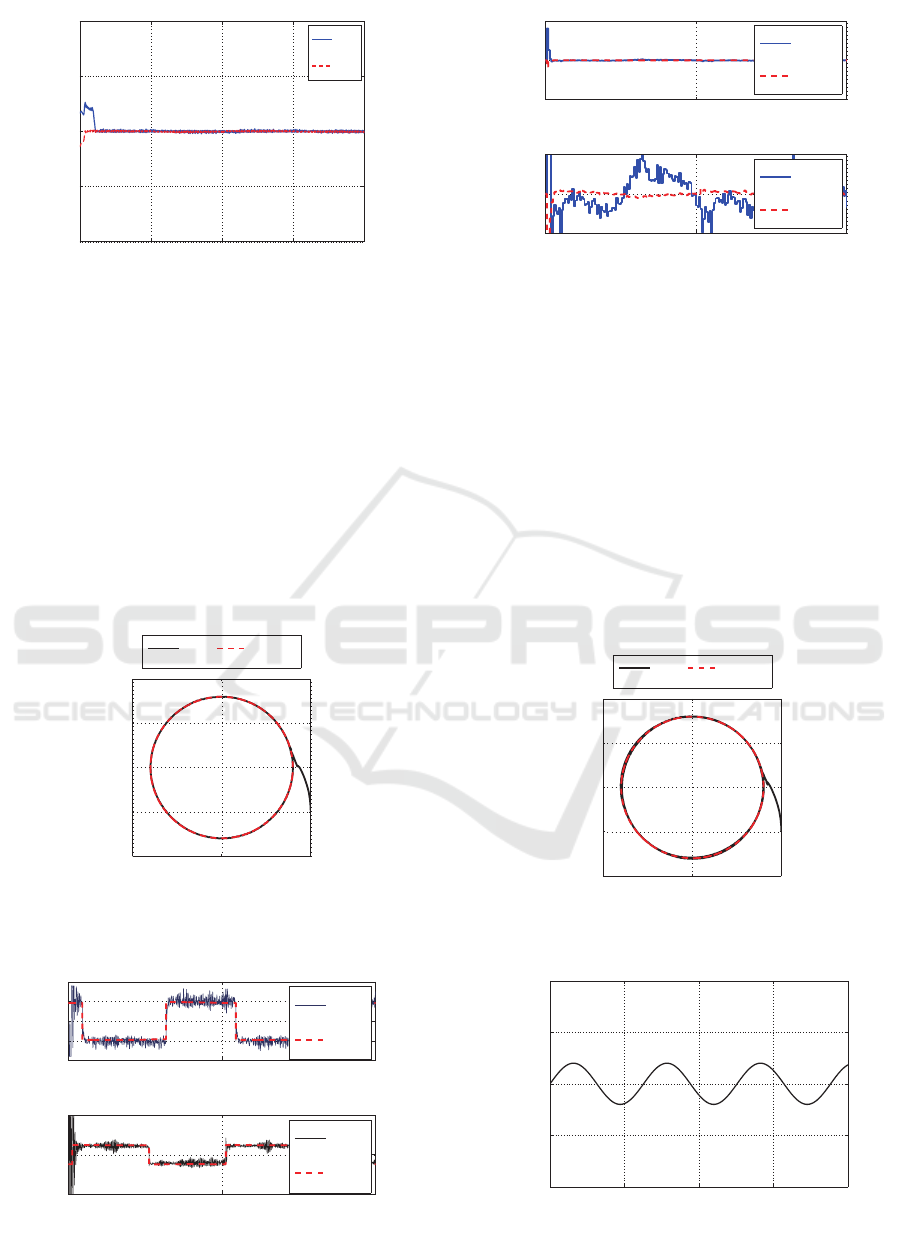
The experimental results are shown in Fig.4 - 14.
The results of the combination of the continuous time
pole placement and the continuous time sliding mode
controller are shown in Fig.4 - 6. The response of
the end portion of the manipulator and the control in-
put signals are shown in Fig.4 and Fig.5, respectively.
The responses of σ
1
and σ
2
are shown in Fig.6 which
̻
;>P@
<>P@
b
b
;<
;
<
Figure 4: Control Response and Desired Trajectory of the
End Portion.
̻
̻
7LPH>VHF@
τ
W>1P@
b
b
τ
W
τ
W
̻
7LPH
>
VHF
@
τ
W>1P@
b
b
τ
W
τ
W
Figure 5: Control Input u(t).
ICINCO 2016 - 13th International Conference on Informatics in Control, Automation and Robotics
444
̻
̻
7LPH>VHF@
σW
b
b
σ
W
σ
W
Figure 6: Response of σ
1
(t) and σ
2
(t).
implies the sliding mode control works well. How-
ever, as shown in Fig.5, the continuous sliding mode
controller has chattering problem.
Fig.7 - 9 show the experimental results of the com-
bination of the continuous time pole placement and
the discrete sliding mode controller with η
i
= 1. The
response of the end portion of the manipulator and
the control input signals are shown in Fig.7 and Fig.8,
respectively. The responses of σ
1
and σ
2
are shown
in Fig.9 which implies the sliding mode control also
works well. Compare to the continuous sliding mode
̻
;>P@
<>P@
b
b
;<
;
<
Figure 7: Control Response and Desired Trajectory of the
End Portion.
̻
̻
7LPH>VHF@
τ
W>1P@
b
b
τ
W
τ
W
̻
7LPH
>
VHF
@
τ
W>1P@
b
b
τ
W
τ
W
Figure 8: Response of ∆u(t).
̻
7LPH>VHF@
σ >N@
b
b
σ
>N@
σ
>N@
̻
7LPH
>
VHF
@
σ >N@0DJQLILHG
b
b
σ
>N@
σ
>N@
Figure 9: Response of x(t).
case, the chattering of the discrete version of the slid-
ing mode control is very small.
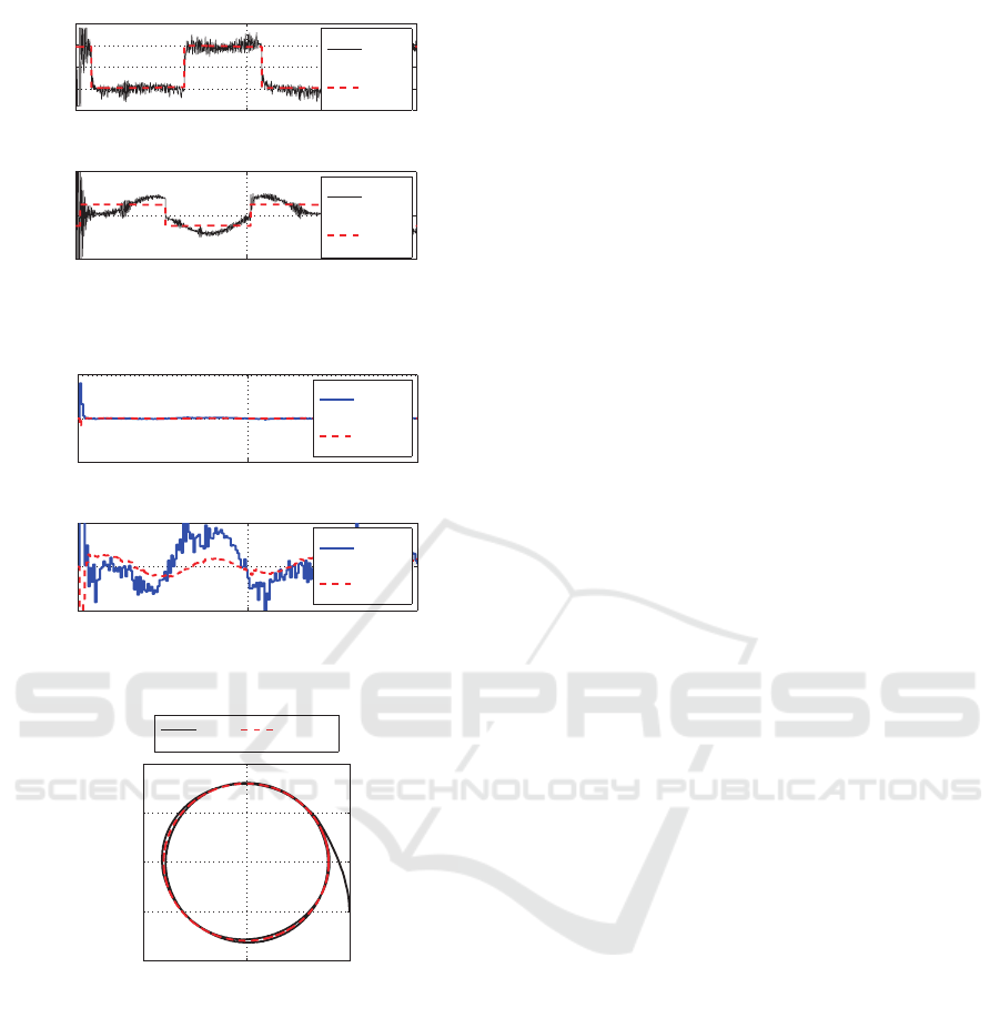
The experimental results of the same controller
(the discrete version) with a disturbance are shown in
Fig.10-13. The response of the end portion of the ma-
nipulator is shown in Fig.10. In this experiment, the
disturbance in Fig.11 is added to the input channel.
The control input signals is shown in Fig.12. And,
the responses of σ
1
and σ
2
are shown in Fig.13.
Fig.14 shows the response of the end portion of
the manipulator with only the pole placement con-
troller with the same disturbance as the previous case.
̻
;>P@
<>P@
b
b
;<
;
<
Figure 10: Response of ∆x(t).
̻
̻
7LPH>VHF@
KWb>1P@
Figure 11: Response of ∆u(t).
Experimental Results of Trajectory Tracking Control of Robot Manipulator using Time Varying Sliding Mode Controller
445
̻
̻
7LPH>VHF@
τ
W>1P@
b
b
τ
W
τ
W
̻
7LPH
>
VHF
@
τ
W>1P@
b
b
τ
W
τ
W
Figure 12: Response of x(t).
̻
7LPH>VHF@
σ
>N@
b
b
σ
>N@
σ
>N@
̻
7LPH
>
VHF
@
σ
>N@0DJQLILHG
b
b
σ
>N@
σ
>N@
Figure 13: Response of ∆u(t).
̻
;>P@
<>P@
b
b
;<
;
<
Figure 14: Response of ∆u(t).
The controller with only the pole placement also has
a good performance under the disturbance, but, if we
need high accuracy performance, the combination of
the continuouspole placement and the discrete sliding
mode control is one practical choice for the trajectory
tracking control of a practical nonlinear systems.
6 CONCLUSIONS
In this paper, the design procedure of sliding mode
controller for linear time-varying system is presented.
For this purpose, the time-varying pole placement
feedback is used so that the closed loop system is
equivalent to some linear time invariant system. Then,
the conventional design method of the sliding mode
control can be applied to this time invariant system.
In this paper, this controller is applied to the actual 2-
link robot manipulator, and experimental results were
shown. The results show the controller has a good
performance with high accuracy under disturbance.
REFERENCES
Chi-Tsong Chen (1999)C Linear System Theory and Design
(Third edition). OXFORD UNIVERSITY PRESS
Charles C. Nguyen (1987)C Arbitrary eigenvalue assign-
ments for linear time-varying multivariable control
systems. International Journal of Control, 45, 1051–
1057
W.J.Rugh (1993) Linear System Theory 2nd Edition pren-
tice hall
Y.Mutoh (2011)C A New Design Procedure of the Pole-
Placement and the State Observer for Linear Time-
Varying Discrete Systems. Informatics in Control, Au-
tomation and Robotics, p.321-334, Springer
Michael Val´aˇsek (1995)C Efficient Eigenvalue Assignment
for General Linear MIMO systems. Automatica, 31-
11, 1605–1617
Y.Mutoh and Kimura (2011)C Observer-Based Pole Place-
ment for Non-Lexicographically-fixed Linear Time-
Varying Systems. 50th IEEE CDC and ECC
V.Utkin (1992), Sliding Mode in Control and Optimization,
Springer-Verlag
Y.Mutoh and N.Kogure(2014), Sliding Mode Control of
Linear Time-Varying Systems, The 11th ICINCO
ICINCO 2016 - 13th International Conference on Informatics in Control, Automation and Robotics
446
