Augmented Postprocessing of the FTLS Vectorization Algorithm

Approaching to the Globally Optimal Vectorization of the Sorted Point Clouds

Ales Jelinek and Ludek Zalud

Department of Control and Instrumentation, Brno University of Technology, Technicka 12, Brno, Czech Republic

Keywords:

Vectorization, Point Cloud, Linear Regression, Least Squares Fitting, Mobile Robotics.

Abstract:

Vectorization is a widely used technique in many areas, mainly in robotics and image processing. Appli-

cations in these domains frequently require both speed (for real-time operation) and accuracy (for maximal

information gain). This paper proposes an optimization for the high speed vectorization methods, which leads

to nearly optimal results. The FTLS algorithm uses the total least squares method for ﬁtting the lines into the

point cloud and the presented augmentation for the reﬁnement of the results, is based on a modiﬁed Nelder-

Mead method. As shown on several experiments, this approach leads to better utilization of the information

contained in the point cloud. As a result, the quality of approximation grows steadily with the number of

points being vectorized, which was not achieved before. Performance costs are still comparable to the original

algorithm, so the real-time operation is not endangered.

1 INTRODUCTION

Vectorization is a process, which produces some kind

of geometrical primitive (line segment, arc, polyno-

mial curve) which describes a general shape of a given

set of data points. This procedure has several advan-

tages.

At ﬁrst, vectorization converts the discrete mea-

surements into their continuous abstraction. This ef-

fect is used in mobile robotics, where laser scanners

are used for sensing of the environment around the

robot. After the measurement, the point cloud is vec-

torized and utilized during the map building process

(Nguyen et al., 2007). This is an important task of var-

ious mobile robots, especially of those dedicated to

exploration and reconnaissance (Zalud et al., 2008).

Very similar problem is the 3D surface or infrastruc-

ture reconstruction (Xu et al., 2015) from the airborne

LiDAR used in cartography. Computer vision and im-

age processing applications also take advantage of the

vectorization in various applications, such as shape

detection (Mathibela et al., 2013) and photogramme-

try (Liu et al., 2011). Another contextual domain of

application is trajectory tracking (Werner et al., 2014)

and infrastructure networks mapping, such as roads in

(Xiangyun Hu et al., 2014).

Second, the vectorization process has a general-

ization ability, which reduces noise and negligible de-

tails in the measurement. Noise reduction is very use-

ful in precise laser scanning applications, requiring

minimal error (Heinz et al., 2001). Filtration of the

negligible details is widely used in cartography, where

different levels of details are obtained with varying

settings of the vectorizing algorithm (Shi and Cheung,

2006).

The third important feature of a vectorized data

set is the reduction of the amount of the data stored.

In a typical application with thousands of measured

points converted into units or tens of line segments,

the memory savings of two orders of magnitude can

be easily observed. This fact is mainly utilized in

cartography, where large maps have to be stored ef-

ﬁciently (Kandal and Karschti, 2014).

The examples summarized in the previous para-

graphs clearly show, that the vectorization has a wide

usage across a variety of scientiﬁc and technical do-

mains. There are some applications, which are not

time critical, but in general, the faster and more ac-

curate the vectorization algorithm is, the higher is its

suitability for practical applications. The motivation

of the presented research is to devise a method, which

would be fast enough for the real-time applications in

robotics and image processing and which would pro-

vide results with the maximal accuracy. At the cost of

slightly reduced speed of the original algorithm, the

further described method fulﬁls this objective.

216

Jelinek, A. and Zalud, L.

Augmented Postprocessing of the FTLS Vectorization Algorithm - Approaching to the Globally Optimal Vectorization of the Sorted Point Clouds.

DOI: 10.5220/0005962902160223

In Proceedings of the 13th International Conference on Informatics in Control, Automation and Robotics (ICINCO 2016) - Volume 2, pages 216-223

ISBN: 978-989-758-198-4

2 STATE OF THE ART

There are plenty of vectorization methods described

in the literature. Various approaches are devised

for different situations, but the two main categories,

which can be distinguished, differ in the nature of the

input data. The general algorithms accept any arbi-

trary set of data points, but this advantage is redeemed

by a larger computational complexity. The second

category of the algorithms works only on the sorted

data, but usually performs much faster.

In the following text, we are going to speak about

the ”optimality” of vectorization and the ”globally op-

timal” results. Since every vectorization algorithm

employs some error function to enumerate quality of

the approximation, optimal result is achieved, when

this function reaches its minimum. Global optimality

is used to emphasize minimization of the error func-

tion for the whole data set, not just a single line seg-

ment.

2.1 General Algorithms

General algorithms are able to produce globally opti-

mal results, or resemble optimality at least. For exam-

ple, Hough transformation (Hough, 1962) in its clas-

sical implementation relies on the systematic search

through the whole state space of possible solutions.

This process can be enhanced (Norouzi et al., 2009)

to focus on the most promising areas, which might

result in globally optimal vectorization. Another pop-

ular method is RANSAC (Fischler and Bolles, 1981),

which is based on random sampling of the data set.

With enough iterations and luck, it converges to glob-

ally optimal solution as well. Another examples

are optimization techniques, suited for highly com-

plex problems, such as genetic algorithms (Mirmehdi

et al., 1997).

The paper (Nguyen et al., 2007) proves this kind

of algorithms to be signiﬁcantly slower than the meth-

ods, that we are going to focus on in the rest of this

paper, but for the sake of completeness, since general

algorithms can produce globally optimal results, we

have decided not to omit them.

2.2 Algorithms for the Sorted Data Sets

Sorted data points preserve the information about the

order, in which they come after each other. The

known succession means, that only the consecutive

points can form a single line to be extracted, which

can be exploited to improve performance.

Sometimes the sorted data cannot be obtained, but

for practical situations it is not as constraining, as it

might seem. For example a border in cartography

is by a polyline, where each point has exactly de-

ﬁned neighbours. A similar situation arises in the

laser scanning case as well: the laser usually rotates

around and the distinct measurements are obtained int

the short intervals one after another, so the order is

known as well. In the image processing we can ﬁnd

the edge extracting algorithms, which produce their

results in a form of a chain of the adjacent pixels. All

of these situations are the examples of naturally or-

dered data sets, which makes the algorithms focused

on this type of input very useful.

The simplest and the fastest (Nguyen et al., 2007)

family of algorithms in this category are the point

eliminating (PE) algorithms. A large number of these

methods is described in the literature (Shi and Che-

ung, 2006). The main idea behind them is the elim-

ination of points, which do not carry a crucial in-

formation about the general shape of the point set.

After application of such algorithm, only the most

important points remain, forming a polyline approx-

imating the whole set. Due to loss of informa-

tion from the eliminated points, these methods can-

not provide very accurate results. In the experimen-

tal part of the paper, we have decided to examine

the Reumann-Witkam (RW) algorithm (Reumann and

Witkam, 1974), which has O(n) computational com-

plexity and is probably the fastest vectorization tech-

nique in practical usage. The second PE method,

which will be tested, is the Douglas-Peucker (DP)

algorithm (Douglas and Peucker, 1973), which is

O(nlogn) complex in average and represents a widely

accepted standard in real-time vectorization, being

more accurate than the RW method (Shi and Cheung,

2006), but still very fast (Nguyen et al., 2007).

The second group of the algorithms for vector-

ization of the sorted data is based on the total least

squares (TLS) ﬁtting of the regression line. The main

advantage over the PE methods consists in utiliza-

tion of all of the information contained in the data

set. This leads to higher accuracy, which can effec-

tively suppress the noise. Classical implementation

of the TLS vectorization is the Incremental (INC) al-

gorithm (Nguyen et al., 2007). The optimized version

of the INC algorithm is the Fast Total Least Squares

(FTLS) method (Jelinek et al., 2016). It produces the

same output as the INC algorithm, but signiﬁcantly

faster, especially when a large set of points is being

processed. Both of these methods will be examined

in the experimental section, because INC algorithm

is widely known and FTLS is its recent faster alter-

native. Asymptotic complexity of both algorithms is

O(n). FTLS is also a base for the optimization pro-

posed in this paper.

Augmented Postprocessing of the FTLS Vectorization Algorithm - Approaching to the Globally Optimal Vectorization of the Sorted Point

Clouds

217

2.3 The Problem in the Threshold based

Vectorization

Every vectorization algorithm has an error function.

The general algorithms usually search each line seg-

ment in the data set separately, which leads to min-

imization of the error function in each case. Con-

versely, the algorithms for the sorted data, exploit the

continuity of the given point cloud, traverses through

the data set and set up the break points of the approx-

imating polyline. This approach is prone to give the

nonoptimal results as shows the following example.

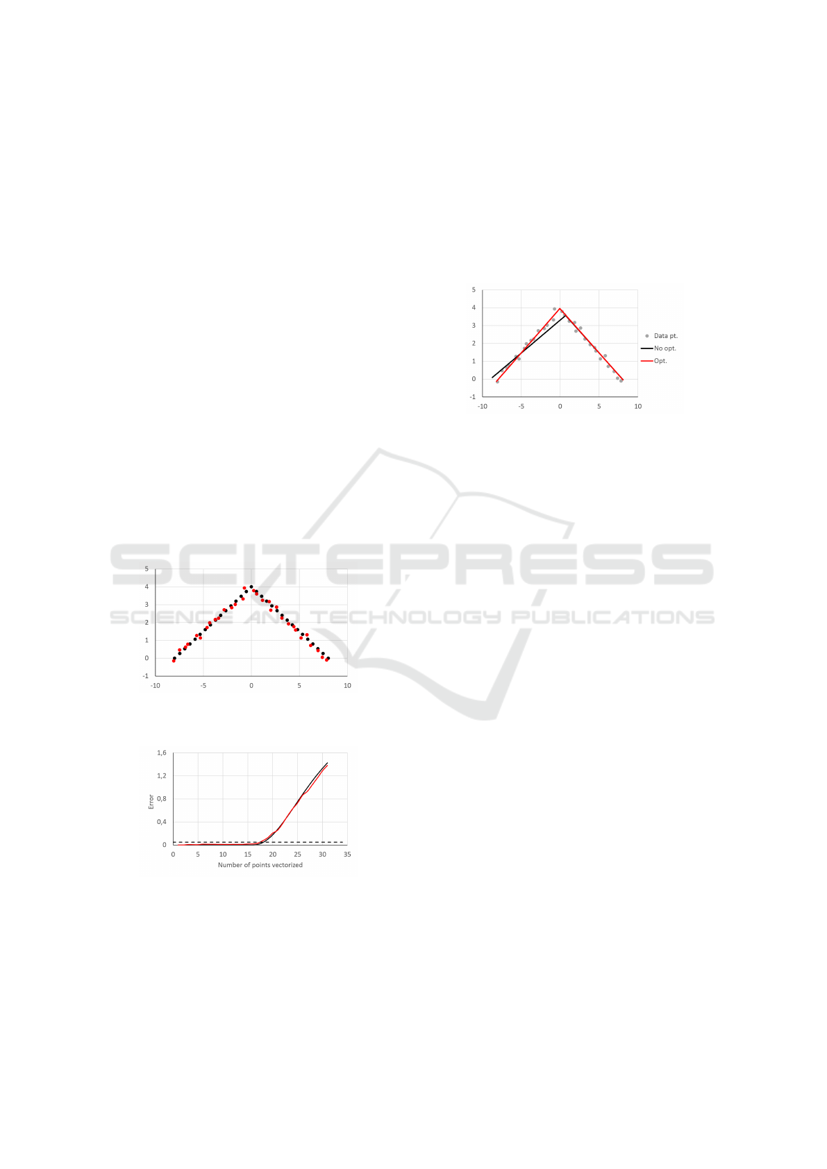
Fig. 1 displays two point clouds: one precise

(black) and one noised (red). Both point clouds are

ordered, as if they were obtained by a laser scanner.

Fig. 2 shows the characteristics of the error function

generated by a TLS method for a given number of

points, counted from the beginning of the cloud. As

expected, the ﬁrst half of the precise point cloud is

vectorized with a zero error, since the points lie ex-

actly in a line. After the midpoint, the error starts to

grow monotonically. Though the whole shape is quite

similar, the ﬁrst half of the red characteristics is cor-

rugated, contains local minima and the break point,

where the error starts to grow rapidly, is not deﬁned

as well as in the previous case.

Figure 1: An example of two simple point clouds. The black

one is precisely generated to form a sharp corner, while the

red one has added a realistic noise.

Figure 2: The error functions generated for the various

number of points from example point clouds in Fig. 1, ob-

tained by the TLS vectorization algorithm. The black char-

acteristics belongs to the precise data set and the red chart

to the noised one. The dashed line illustrates a defensive

choice of a threshold level for a robust vectorization.

All of the fast vectorization methods (whether PE

or TLS) employ a threshold, which is compared to the

error function in each iteration and when exceeded,

the break point is set up and a new approximation is

started. Due to the fact, that the error characteristics

is not ideal, the threshold must be set with appropri-

ate reserve, to ensure robustness and immunity to the

noise. Such a defensive choice of the threshold leads

to higher error than necessary for every line segment

in the approximating polyline, except the last one, as

can be seen in Fig. 3.

Figure 3: Optimal (red) and suboptimal (black) vectoriza-

tion of the noised point cloud (gray). The red and black line

segments approximating the second half of the point cloud

overlap each other.

The negative inﬂuence of the defensively chosen

threshold was slightly magniﬁed for the illustrational

purposes in this case, but even without that, it is a

serious drawback of all of the fast vectorization al-

gorithms. This effect manifests regardless the algo-

rithms traverse the point cloud incrementally (INC

and RW), or perform some sort of an adapted binary

search (FTLS and DP). It is also impossible to sup-

press it by calibration (Kocmanova et al., 2013) or

identiﬁcation (Zalud et al., 2015) of the laser scanner,

because the described problem is an inherent feature

of the TLS and PE algorithms, not a ﬂaw of the input

data. The rest of the paper is focused on minimization

of this unnecessary error.

3 AUGMENTATION OF THE

FTLS ALGORITHM

Globally optimal vectorization of a continuous point

cloud is a really challenging task. There is no prior in-

formation either on the number of line segments in the

approximating polyline, or the position of the break

points. This high degree of uncertainty leads to em-

ployment of the traditional vectorization algorithms

to get an initial guess of the approximation and than

use it for further optimization.

As the primary algorithm, we have chosen the

FTLS algorithm (Jelinek et al., 2016), which is based

o the TLS method and is reasonably fast. The algo-

rithm has three stages of the data processing. The ﬁrst

one produces precomputed sums for every data point

ICINCO 2016 - 13th International Conference on Informatics in Control, Automation and Robotics

218

in the cloud. The data vector belonging to each point

is as follows:

, y

∑

k=1

∑

k=1

∑

k=1

∑

k=1

∑

k=1

(1)

for i = 1. . . N, where N is the number of points be-

ing vectorized. For our purposes, we deﬁne an ad-

ditional vector a

= [0, 0, 0, 0, 0, 0, 0] and form an

augmented data matrix:

A =



. . . a



. (2)

We also deﬁne a submatrix of A as:

A[p, q] =



. . . a



, (3)

determined by the row indices p and q, which follow

the condition 0 ≤ p < q ≤ N.

The second stage of the FTLS algorithm is dedi-

cated to line extraction. The output is an ordered set

of extracted lines, which approximate the whole point

cloud. Every extracted line has an exactly deﬁned in-

terval of points, which belong to it. This information

is used to build a break point vector, where the index

of the last point of every line is stored:

b = [b

, b

, . . . , b

]. (4)

The b

= 0 is a dummy element representing a virtual

point before the beginning of the point cloud. The

last break point always refers to the end of the point

cloud, therefore b

= N. All the other break points

satisfy the condition: b

i−1

< b

for i = 1 . . . L .

Every extracted line has also attached an error

value, which describes, how well the line approxi-

mates the given data. The TLS methods use the vari-

ance of perpendicular distances of points to the line.

The paper (Jelinek et al., 2016) deﬁne it in the follow-

ing manner:

∑

i=1

+ 2ab

∑

i=1

+ b

∑

i=1

− c

(5)

n is the number of points belonging to the line and a,

b and c are the coefﬁcients of a line in a neutral for-

mat: ax + by + c = 0 in XY coordinate system. If a

half-open interval of points (p, q] is given, the sums

can be easily obtained by a simple subtraction of vec-

tors a

and a

. Since the coefﬁcients a, b and c can

be expressed as a function of A[p,q] as well, we can

denote the variance: σ

(A[p, q]).

This adjustment of the notation allows us to ex-

press the error E of the approximation of the whole

point cloud. It is deﬁned as follows:

E(b) =

∑

i=1

(A[b

i−1

, b

])

− b

i−1

. (6)

The original FTLS algorithm does not evaluate any

global error metrics, its third stage consists only in

turning the extracted lines into the polyline, which de-

scribes the general shape of the point cloud. This ap-

proximation is necessarily suboptimal, due to the ef-

fect described in the Subsection 2.3. To get the glob-

ally optimal results analytically, the following set of

the equations would have to be solved:

∂E(b)

∂b

= 0 . . .

∂E(b)

∂b

L−1

= 0. (7)

There is only L − 1 of equations for L extracted lines,

because b

and b

coefﬁcients are deﬁned to be con-

stant, when building the break point vector b ac-

cording to the equation (4). Unfortunately, the an-

alytic solution of the system (7) is extremely com-

plicated or even impossible, because the error func-

tion σ

(A[p, q]) is highly non-linear. It also does not

grow monotonically, which possibly leads to an un-

predictable number of local minima.

To overcome this issue, we have decided to em-

ploy the Nelder-Mead (NM) method (Nelder and

Mead, 1965). It is a non-gradient optimization tech-

nique, which only relies on enumeration of the op-

timized function for various input arguments. This

is a key feature, because thanks to the precomputed

sums of the FTLS algorithm, the evaluation of the

error function is very fast. The NM method is de-

signed for localization of extremes of the non-linear

functions with arbitrary number of arguments. The

method is based on a simplex composed of D+ 1 ver-

tices in a D-dimensional space of possible arguments

of the optimized function. Each vertex has its func-

tion value attached and every iteration the least suit-

able one is replaced by a newly computed successor.

The function value of the new vertex is usually bet-

ter than the previous one, so as the iterations proceed,

the simplex shrinks and closes to the set of arguments

giving the optimal value.

In the original NM method, the simplex is de-

scribed by a set of D + 1 vectors with D elements. In

our case of the search for the optimal break point posi-

tions, the situation is slightly more complex, because

every argument vector for the optimized error func-

tion (6) has constants at the beginning and at the end.

At the beginning of the optimization process, there is

only one initial guess on position of the break points

produced by the second stage of the FTLS algorithm,

therefore L−1 new vertices have to be generated. The

resulting simplex has the structure:

S =



. . . s

L−1



, (8)

Augmented Postprocessing of the FTLS Vectorization Algorithm - Approaching to the Globally Optimal Vectorization of the Sorted Point

Clouds

219

generated by the following rules:

= b,

i, j

= b

i 6= j,

i, j

= b

− τ i = j,

(9)

for i = 1. . . (L − 1) and j = 0 . . . L. As the ﬁrst vertex,

the initial guess is adopted without any changes. The

remaining L − 1 vertices are generated by subtracting

a user deﬁned value τ from a single element of the

vector b (different element for every new vertex). The

τ parameter is an integral variable and should fulﬁl

the condition τ < b

to ensure, that all the elements

of the vertex will satisfy the constraints discussed al-

ready beside the equation (4). τ should correspond

to an expected number of extra points assigned to the

line segment, but the NM method is robust enough to

handle even very rough estimates.

The vertex manipulating operations, which com-

pose the core of every iteration of the NM method,

were implemented in our algorithm according to (La-

garias et al., 1998). The structure of the iteration is

well described, therefore we are not going to repro-

duce the details. The error function (6) and the sim-

plex (8) are enough to start the optimization process.

There are two major differences to the original ap-

proach. The ﬁrst is the introduction of constraints to

otherwise unconstrained method. In general, adding

constraints to the NM method can be very compli-

cated (Le Floc’h, 2012), but in our case, adding limits

cannot lead to worse results, than the initial guess,

neither can cause a collapse of the method. Be-

cause the break points must keep the order deter-

mined by the points in the source point cloud, the

algorithm does not search through the whole (L − 1)-

dimensional space, but only through its part, limited

by the inequality s

i, j−1

< s

i, j

for i = 0 . . . (L − 1) and

j = 1 . . . L. This condition is checked every time af-

ter a new vertex is generated and proceeds from the

end to the beginning of the particular vector. Any

break points out of the range are trimmed to ﬁt into

the boundaries. A new error function value is com-

puted after this check.

The second difference to the original approach is

the discreteness of the arguments of the optimized

function. While the original method is designed to

be used with real numbers, the break points can be

only integers. In combination with the constraints dis-

cussed above, this means, that there is a ﬁnite number

of possible vertices. At the end of the iteration pro-

cess, as the solution becomes more precise, the ver-

tices inevitably start to overlap and the simplex col-

lapses. If that happens, or if the vertices end up in

one hyperplane, the algorithm is stopped and the best

solution is taken as the output of the optimization.

The concept described above ensures, that no

worse result than the initial guess can appear and in

the vast majority of cases a signiﬁcant improvement

can be observed. The postprocessing, after the mod-

iﬁed NM optimization is over, is the same as in the

original FTLS algorithm.

4 EXPERIMENTAL VALIDATION

OF THE METHOD

This section presents several experiments for evalua-

tion of the precision gains and the performance costs

of the augmented FTLS method. For the convenience,

we are going to use the AFTLS abbreviation. Be-

cause the AFTLS method is derived directly from the

FTLS method, we are going to follow the experimen-

tal methodology presented in (Jelinek et al., 2016)

and repeat some benchmarks with the new augmented

vectorization technique. The datasets for the experi-

ments in Fig. 5-8 are directly adopted from (Jelinek

et al., 2016) and so are the illustrational pictures (the

(a) subﬁgure in all of the speciﬁed cases). All of the

measurements are performed again to unify the test

conditions.

All of the algorithms and benchmarks were imple-

mented in the C++ programming language and com-

piled with Microsoft Visual Studio 2012, using the

O2 optimization setting. No other optimizations were

made to keep the tests as general as possible. An in-

terested user of the algorithms may beneﬁt from mul-

tithreaded implementation, SIMD instructions, loop

unrolling and many other techniques, which can im-

prove the performance signiﬁcantly, but are highly

platform dependant. The computer used for running

the benchmarks had a six-core, 64-bit AMD FX-6350

CPU, which runs on 3.9 GHz. Processor cache mem-

ory is large enough to hold all of the data processed

in one iteration.

The metrics used for precision evaluation of the

examined methods is the same as in (Jelinek et al.,

2016), which is based on computation of the error

area demarcated by the true edge and the extracted

polyline approximation. Neither the error metrics for

a single line (5), nor the error function for the whole

continuous point cloud (6), used during the vectoriza-

tion process, are suitable, because both of them ap-

parently cannot take into account the real edges.

The ﬁrst tested case is shown in Fig. 4a. The con-

tinuous parts of the point cloud can be approximated

by a single line, which is a perfect situation for com-

parison of the PE and the TLS based methods. From

the precision benchmark in Fig. 4b it is clear, that the

PE methods are not capable to utilize the information

ICINCO 2016 - 13th International Conference on Informatics in Control, Automation and Robotics

220

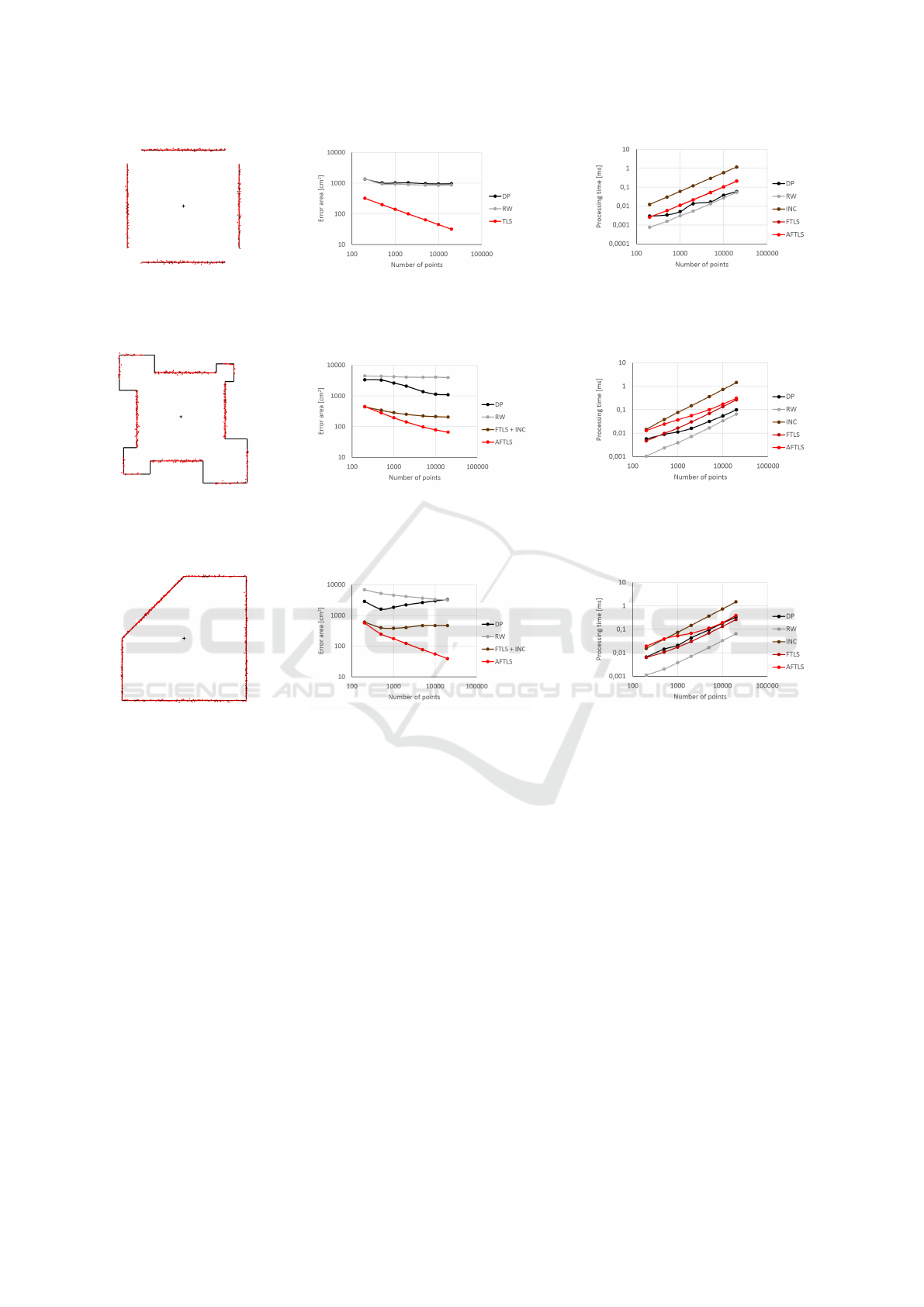
(a) The point cloud. (b) The precision benchmark. (c) The speed benchmark.

Figure 4: An example of a simple point cloud where no break points are present. All of the TLS based methods provide the

same precision of vectorization and the FTLS and AFTLS algorithms exhibit the same speed.

(a) The point cloud. (b) The precision benchmark. (c) The speed benchmark.

Figure 5: This example consists of eight continuous parts, four of which contain one break point and four is straight without

bending. The AFTLS algorithm provides the most accurate results.

(a) The point cloud. (b) The precision benchmark. (c) The speed benchmark.

Figure 6: The continuous point cloud examined in this experiment has four bendings. As the number of break points in the

cloud increases, the advantage of the AFTLS method becomes even more evident.

from all of the processed points, while the TLS meth-

ods use it to gradually reﬁne the results as the num-

ber of points grows. The speed benchmark in Fig. 4c

proves, that there is no performance penalty of the

AFTLS algorithm, if no break points are present.

The second, example in Fig. 5a contains straight

lines and polylines with one break point. The FTLS

and INC algorithms, although TLS based and signif-

icantly more accurate than the PE methods, cannot

lower the error under certain threshold, because of

the problem discussed in Section 2.3. The AFTLS al-

gorithm effectively solves this issue and provides the

better results, the higher is the amount of the input

points (see Fig. 5b). Computational costs are evident

from the speed benchmark in Fig. 5c. The relative

performance loss decreases with the number of points

being processed.

The shape of the point cloud depicted in Fig. 6a

leads to even stronger manifestation of effects dis-

cussed in the previous paragraph. AFTLS keeps to

reﬁne the output polyline with the growing number of

processed points as before (see Fig. 6b) and the speed

sticks close to the FTLS characteristics as well (see

Fig. 6c). We have not deeply examined the behaviour

of the DP and the RW precision characteristics ob-

servable in Fig. 5b and Fig. 6b, because the paper is

focused on the AFTLS algorithm. We believe, it orig-

inates from the hidden regularities in the point cloud

generator, which are related to the given number of

points. Nevertheless, the fact that the PE methods are

not able to utilize the information from the eliminated

points can still be considered valid.

The last two experiments shown in Fig. 7 and

Fig. 8 are virtual simulations of an environment,

which is commonly encountered by a mobile robots.

Results are similar and correspond to the ﬁndings

Augmented Postprocessing of the FTLS Vectorization Algorithm - Approaching to the Globally Optimal Vectorization of the Sorted Point

Clouds

221

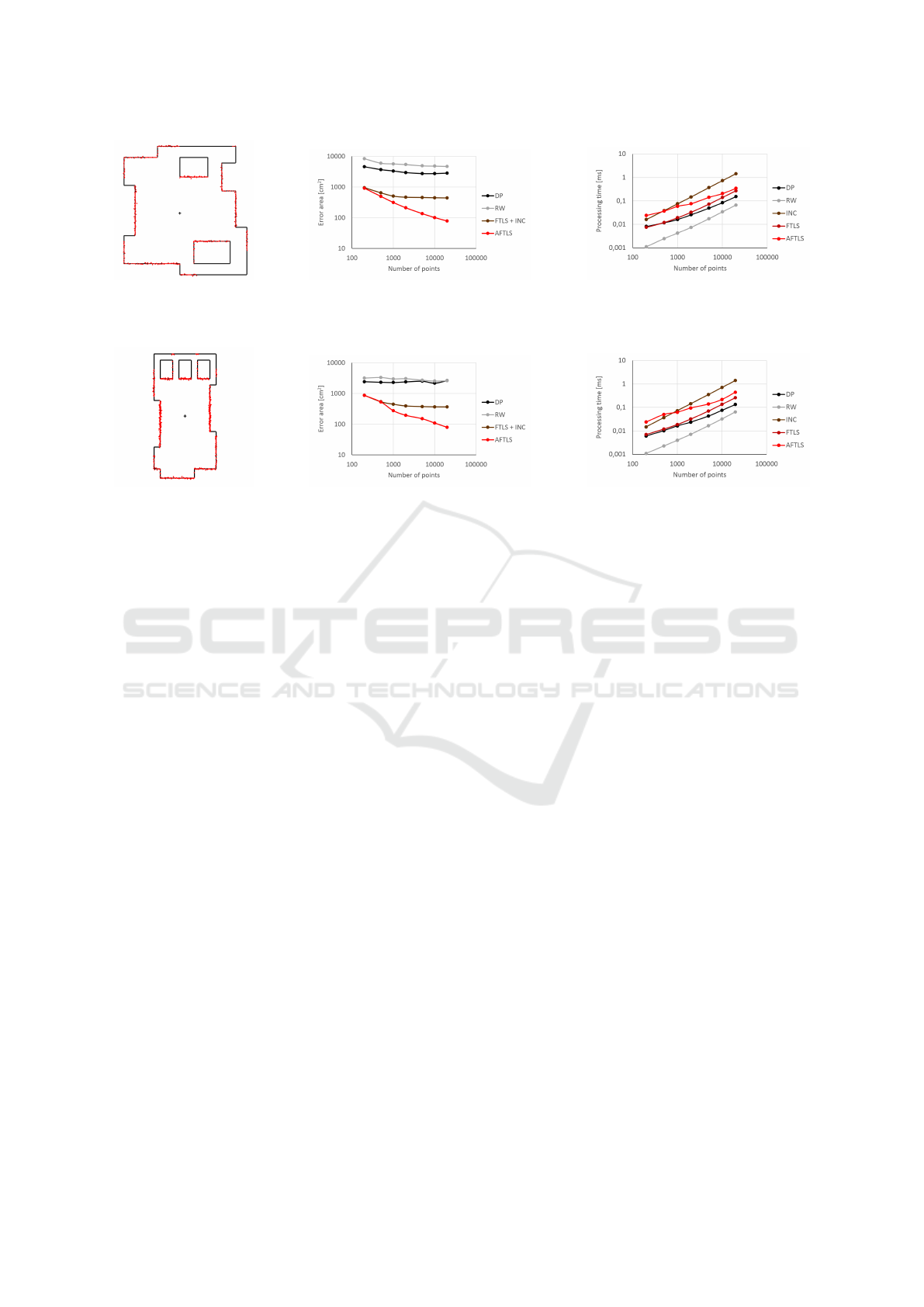
(a) The point cloud. (b) The precision benchmark. (c) The speed benchmark.

Figure 7: The point cloud obtained in a virtually simulated environment. The AFTLS algorithm provides the most precise

approximations, while the speed is comparable (yet lower) to the other algorithms.

(a) The point cloud. (b) The precision benchmark. (c) The speed benchmark.

Figure 8: Another example of a virtual environment similar to real world cases. The results correspond to the expectations

about behaviour of the tested algorithms.

from the previous experiments. The AFTLS method

consistently delivers the most accurate results. For

point clouds with lower number of points, the pre-

cision gain is small and relative computational cost

high in comparison with the FTLS method, but for

the dense point clouds, it is deﬁnitely worthwhile.

Experimenting with the real laser scans was found

to be very complicated. The ﬁrst issue is a limited

number of the output points of the laser scanners

available these days. The Velodyne HDL 32, that we

have used for testing, delivers ca. two thousands of

points per scan. This is right enough to see the ben-

eﬁts of the AFTLS method, but the most signiﬁcant

results are expected in the future, with more output

points. The second big issue is the precision of the

reference measurement for the precision benchmark-

ing. Every millimetre in the reference measurement

taken in an empty room, had a serious impact on the

error enumeration, which could easily cause the mis-

leading results. We have tested only the speed on real

data, which was proved to be in perfect agreement

with simulations in Fig. 7a and 8a. The same we ex-

pect for accuracy.

5 CONCLUSIONS

This paper proposes a new approach to fast vectoriza-

tion of the sorted point clouds. The presented method

originates from the FTLS algorithm, which is based

on the TLS line ﬁtting, therefore it can utilize the in-

formation from every processed point in the cloud.

It also incorporates an optimization mechanics based

on a modiﬁed Nelder-Mead method, to overcome the

general problem of the fast, threshold based, vector-

ization techniques. Since the optimization is based

on the NM method and the function for estimation

of the global error of the approximation is not guar-

anteed to have a single minimum, we cannot claim

the method to be truly globally optimal. On the other

hand, the algorithm with this augmentation is able to

reﬁne the vectorization results and approach the glob-

ally optimal solution very close. The results of several

experiments have proved, that the augmented FTLS

algorithm signiﬁcantly enhances precision of the ap-

proximation of the point cloud, especially of the most

dense ones containing many thousands of points. This

fact is really promising, because the laser scanners

with higher point densities can be expected in the near

future.

Further research in this ﬁeld is going to be fo-

cused on effective implementation of the algorithm on

a special hardware architectures and the deployment

to the practical applications, which could take advan-

tage of a fast and highly precise vectorization, such as

robotics and machine vision.

ACKNOWLEDGEMENTS

The grant No. FEKT-S-14-2429 - ”The re-

search of new control methods, measurement pro-

ICINCO 2016 - 13th International Conference on Informatics in Control, Automation and Robotics

222

cedures and intelligent instruments in automation”

ﬁnancially supported by the Internal science fund

of BUT. The Department of Control and Instru-

mentation (BUT - FEEC). The project CEITEC

(CZ.1.05/1.1.00/02.0068), ﬁnanced from the Euro-

pean Regional Development Fund and by the TACR

under the project TE01020197 - CAK3.

REFERENCES

Douglas, D. H. and Peucker, T. K. (1973). Algorithms for

the Reduction of the Number of Points Required to

Represent a Digitized Line or its Caricature. Carto-

graphica: The International Journal for Geographic

Information and Geovisualization, 10(2):112–122.

Fischler, M. A. and Bolles, R. C. (1981). Random sample

consensus: a paradigm for model ﬁtting with appli-

cations to image analysis and automated cartography.

Communications of the ACM, 24(6):381–395.

Heinz, I., Hartl, F., and Frohlich, C. (2001). Semi-

automatic 3D CAD model generation of as-built con-

ditions of real environments using a visual laser radar.

In Proceedings 10th IEEE International Workshop

on Robot and Human Interactive Communication.

ROMAN 2001 (Cat. No.01TH8591), pages 400–406.

IEEE.

Hough, P. V. C. (1962). Method and Means for Recognizing

Complex Patterns.

Jelinek, A., Zalud, L., and Jilek, T. (2016). Fast total least

squares vectorization. Journal of Real-Time Image

Processing.

Kandal, P. and Karschti, S. (2014). Method for simpliﬁed

storage of data representing forms.

Kocmanova, P., Zalud, L., and Chromy, A. (2013). 3D prox-

imity laser scanner calibration. In 2013 18th Interna-

tional Conference on Methods & Models in Automa-

tion & Robotics (MMAR), pages 742–747. IEEE.

Lagarias, J. C., Reeds, J. a., Wright, M. H., and Wright, P. E.

(1998). Convergence Properties of the Nelder–Mead

Simplex Method in Low Dimensions. SIAM Journal

on Optimization, 9(1):112–147.

Le Floc’h, F. (2012). Issues of Nelder-Mead Simplex Opti-

misation with Constraints. SSRN Electronic Journal,

pages 1–7.

Liu, Z., Zhang, B., Li, P., Guo, H., and Han, J. (2011).

Automatic registration between remote sensing image

and vector data based on line features. In 2011 19th

International Conference on Geoinformatics, number

2008, pages 1–5. IEEE.

Mathibela, B., Posner, I., and Newman, P. (2013). A road-

work scene signature based on the opponent colour

model. In 2013 IEEE/RSJ International Conference

on Intelligent Robots and Systems, pages 4394–4400.

IEEE.

Mirmehdi, M., Palmer, P. L., and Kittler, J. (1997). Robust

line segment extraction using genetic algorithms. In

Image Processing and Its Applications, 1997., Sixth

International Conference on, volume 1, pages 141 –

145 vol.1. IEEE.

Nelder, J. A. and Mead, R. (1965). A Simplex Method

for Function Minimization. The Computer Journal,

7(4):308–313.

Nguyen, V., G

achter, S., Martinelli, A., Tomatis, N., and

Siegwart, R. (2007). A comparison of line extrac-

tion algorithms using 2D range data for indoor mobile

robotics. Autonomous Robots, 23(2):97–111.

Norouzi, M., Yaghobi, M., Siboni, M., and Jadaliha, M.

(2009). Recursive line extraction algorithm from 2d

laser scanner applied to navigation a mobile robot. In

2008 IEEE International Conference on Robotics and

Biomimetics, pages 2127–2132. IEEE.

Reumann, K. and Witkam, A. P. M. (1974). Optimiz-

ing Curve Segmentation in Computer Graphics. In

Proceedings of International Computing Symposium,

pages 467–472, Amsterdam. North-Holland Publish-

ing Company.

Shi, W. and Cheung, C. (2006). Performance Evaluation

of Line Simpliﬁcation Algorithms for Vector General-

ization. The Cartographic Journal, 43(1):27–44.

Werner, M., Schauer, L., and Scharf, A. (2014). Reliable

trajectory classiﬁcation using Wi-Fi signal strength in

indoor scenarios. In 2014 IEEE/ION Position, Loca-

tion and Navigation Symposium - PLANS 2014, pages

663–670. IEEE.

Xiangyun Hu, Yijing Li, Jie Shan, Jianqing Zhang, and

Yongjun Zhang (2014). Road Centerline Extraction in

Complex Urban Scenes From LiDAR Data Based on

Multiple Features. IEEE Transactions on Geoscience

and Remote Sensing, 52(11):7448–7456.

Xu, C., Frechet, S., Laurendeau, D., and Miralles, F. (2015).

Out-of-Core Surface Reconstruction from Large Point

Sets for Infrastructure Inspection. In 2015 12th Con-

ference on Computer and Robot Vision, pages 313–

319. IEEE.

Zalud, L., Kocmanova, P., Burian, F., Jilek, T., Kalvoda, P.,

and Kopecny, L. (2015). Calibration and Evaluation

of Parameters in A 3D Proximity Rotating Scanner.

Elektronika ir Elektrotechnika, 21(1):3–12.

Zalud, L., Kopecny, L., and Burian, F. (2008). Orpheus

Reconnissance Robots. In 2008 IEEE International

Workshop on Safety, Security and Rescue Robotics,

number October, pages 31–34. IEEE.

Augmented Postprocessing of the FTLS Vectorization Algorithm - Approaching to the Globally Optimal Vectorization of the Sorted Point

Clouds

223