Mobile Application Usage Concentration in a Multidevice World

Benjamin Finley

, Tapio Soikkeli

and Kalevi Kilkki

Department of Communications and Networking, Aalto University, Otakaari 5, Espoo, Finland

Verto Analytics, Innopoli 2, Tekniikantie 14, Espoo, Finland

Keywords:

Mobile Applications, Device Based Monitoring, Mobile Usage.

Abstract:

Mobile applications are a ubiquitous part of modern mobile devices. However the concentration of mobile

application usage has been primarily studied only in the smartphone context and only at an aggregate level. In

this work we examine the app usage concentration of a detailed multidevice panel of US users that includes

smartphones, tablets, and personal computers. Thus we study app usage concentration at both an aggregate

and individual device level and we compare the app usage concentration of different device types. We detail

a variety of novel results. For example we show that the level of app usage concentration is not correlated

between smartphones and tablets of the same user. Thus extrapolation between a user’s devices might be

difﬁcult. Overall, the study results emphasize the importance of a multidevice and multilevel approach.

1 INTRODUCTION

The rise of the smartphone has led to the mobile ap-

plication (app) as a basic and ubiquitous part of mo-

bile device usage. This ubiquity implies that un-

derstanding mobile app usage in general is impor-

tant for the entire mobile ecosystem. Furthermore,

the widespread use of smartphones in daily life sug-

gests that mobile app usage is interesting to an array

of broader ﬁelds (such as media theory). In light of

this, mobile app usage has been studied by many re-

searchers (Falaki et al., 2010; B

ohmer et al., 2011; Xu

et al., 2011; Soikkeli et al., 2013; Jung et al., 2014;

Hintze et al., 2014).

Mobile app studies have often examined basic us-

age statistics such as mean app session length and

transition probabilities between apps (B

ohmer et al.,

2011; Soikkeli et al., 2013). However despite the

large volume of apps available from curated apps

stores, relatively few studies have examined the con-

centration of usage across apps

. Furthermore, stud-

ies that have examined app usage concentration have

analyzed only aggregate level smartphone usage (typ-

ically because tablet or other device type usage is not

available) (Jung et al., 2014).

Note that by the term concentration of usage we mean the

concentration of the distribution of total time across mo-

bile apps. Such concentration can be on an individual (time

of an individual distributed among their apps) or aggre-

gate level (total time of all individuals distributed among

all apps)

Contrastingly, in this study we aim to provide

a holistic view of mobile app usage concentration.

Speciﬁcally, we examine the app usage concentration

for a highly granular multidevice panel that includes

smartphones, tablets, and personal computers (PC).

Thus we can study and compare app usage concen-

tration levels for different device types at both the ag-

gregate (market) level and individual device level. In

addition, because the panel contains users with multi-

ple devices in the panel we can determine if measures

such as the Theil index (a concentration measure) or

the number of utilized apps are correlated between de-

vices of the same user.

In summary, we enumerate the following novel

contributions:

1. We show that, on an aggregate level, app usage

is highly concentrated on all three device types

(smartphone, tablet, and PC) but that signiﬁcant

differences in app usage concentration between

the device types still exist. These differences re-

sult partly from differences in the types (cate-

gories) of apps typically utilized with each device

type.

2. We show that, on the device level, there are large

variations in app usage concentration within all

device types. In other words characterizing the

typical user’s app usage concentration is difﬁcult.

3. We show that app usage concentration is not cor-

related in cases of smartphone and tablet, smart-

phone and PC, or tablet and PC of the same user.

Finley, B., Soikkeli, T. and Kilkki, K.

Mobile Application Usage Concentration in a Multidevice World.

DOI: 10.5220/0005964000400051

In Proceedings of the 13th International Joint Conference on e-Business and Telecommunications (ICETE 2016) - Volume 6: WINSYS, pages 40-51

ISBN: 978-989-758-196-0

Therefore, extrapolation of app usage concentra-

tion between devices of the same user might be

difﬁcult.

4. We show that the total number of utilized

apps is signiﬁcantly negatively correlated (r =

−0.304, p ≤ 0.05) between PCs and tablets of

the same user, weakly positively correlated (r =

0.146) between tablets and smartphones of the

same user, and not correlated (r = −0.024) be-

tween smartphones and PCs of the same user.

We relate the signiﬁcant negative correlation be-

tween PCs and tablets to device type substitu-

tion. Whereas a further exploration of smartphone

and tablet app usage ﬁnds that only a relatively

small fraction (~17%) of a user’s total mobile apps

(union of apps on their smartphone and tablet)

are actually utilized on both their smartphone and

tablet.

Overall the concentration of app usage has theoreti-

cal and practical implications in several ﬁelds. For

example, app usage concentration has been linked to

media repertoire theory and more general concepts of

media usage concentration (Jung et al., 2014). As an

example in terms of entertainment apps, users do not

access all of their entertainment apps randomly and

for random lengths of time but rather respond to the

problem of choice by creating a repertoire or subset

of entertainment apps to utilize frequently. Then habit

formation reinforces these choices over time leading

to concentration.

Furthermore, beyond theory, app usage and usage

concentration are important in the area of mobile ad-

vertising. For example, our research on app usage

across devices of the same user could help in devel-

oping models of multidevice in-app advertisement ex-

posure and in understanding the mobile advertising

landscape more generally.

2 BACKGROUND

2.1 Concentration Measures

The concentration or dispersion of a resource (such

as money, or in our case user time) can be character-

ized by a large number of different measures such as

the Gini coefﬁcient. These measures have primarily

been utilized by economists to compare income and

wealth inequality. In this work we utilize two distinct

concentration measures: the Gini coefﬁcient and the

Theil index. We utilize the Gini coefﬁcient because

it is the most well known and widely reported mea-

sure. While we utilize the Theil index because it has

stronger theoretical underpinnings in information the-

ory. In addition the Theil index is more sensitive to

large tail values than the Gini coefﬁcient and thus is

complementary (Cowell and Flachaire, 2007).

The Gini coefﬁcient is based on the concept of the

Lorenz curve, an empirical curve on the plot of the cu-

mulative proportion of the population versus the cu-

mulative proportion of a variable distributed among

that population (such as income). The Gini coefﬁcient

is then the area between the Lorenz curve and the per-

fectly equal distribution curve (of 45 degrees) divided

by the total area under the equal distribution curve.

The Gini coefﬁcient has a range of [0, 1] indicating

minimum and maximum concentration respectively.

The standard Gini coefﬁcient formulation we utilize

is shown in Equation 1 where n is the total number

of apps, y

is total usage time in seconds for app i,

i = 1, . . . , n indicates the total app usage times y

as or-

der statistics (in other words y

≤ y

≤ · ·· ≤ y

and ¯y is the mean usage time for an app (Cowell and

Flachaire, 2014).

G =

∑

i=1



2i − n − 1

¯y · n(n − 1)



(1)

The Theil index is derived from information theory

and represents the maximum theoretical entropy of

data minus the actual data entropy (Theil, 1967). The

Theil index formulation we utilize (known as the

Theil-T redundancy) is detailed in Equation 2 where

where n is the total number of apps, y

is total us-

age time in seconds for app i, and ¯y is the mean usage

time for a single app. This formulation includes a nor-

malization of

lnn

so that the Theil index is a relative

rather than absolute inequality measure and compar-

isons between data with different numbers of groups

(in our case apps) are feasible (Roberto, 2015). This

normalized Theil index has a range of [0, 1] indicating

minimum and maximum concentration respectively.

T =

n · lnn

∑

i=1



¯y

· ln

¯y



(2)

2.2 Aggregate and Device Levels, and

Utilized Apps

We brieﬂy deﬁne the aggregate level and device level

of analysis.

In the aggregate level of analysis, we aggregate

(sum) the total usage of each app over all devices of

a given platform-device type combination. As an ex-

ample, in the aggregate iOS tablet case each app value

is the total usage of that app from all iOS tablets. We

utilize platform-device type combinations instead of

simply device types because app packages are plat-

form speciﬁc and the same app typically has different

Mobile Application Usage Concentration in a Multidevice World

package names on iOS and Android. Thus instead of

smartphone, tablet, and PC, we have Android smart-

phone, iOS smartphone, Android tablet, iOS tablet,

and PC.

In the device level of analysis, we examine the app

usage for only that individual given device. We can

still group these individual devices based on platform-

device type combinations but importantly each device

will have, for example, a Gini coefﬁcient based on

that device’s app usage.

Finally, we note that all of our analysis looks at us-

age concentration of utilized apps. In other words, we

do not include apps that are installed but not utilized

at all in the one month observation period.

3 PANEL DATA

The main data are several subsets of a large user panel

arranged by Verto Analytics

in the United States

in February 2015 (one month observation period).

Panelists were recruited online and were surveyed

through an initial recruitment survey to determine the

devices they own. Panelists were then instructed to in-

stall custom monitoring apps to all of their applicable

devices (speciﬁcally their smartphone, tablet, and/or

PC). Only panelists that installed the monitoring apps

to all their applicable devices were considered for the

panel. The monitoring apps log events such as an app

moving to the foreground or background of the dis-

play and HTTP network requests. All panelists were

paid for participation. All provided user data was

anonymized with no personally identifying informa-

tion.

In terms of extracting subsets of data we utilize

the notion of active panelists. We deﬁne a panelist

as active with a given device if the length between

their ﬁrst usage of the month and last usage of the

month for that device is at least 23 days. The num-

ber of active panelists for each platform-device type

combination are detailed in Table 2. The number of

active panelists with two device types in the panel (in-

dicating that the user is active with both devices) are

detailed in Table 3. All analysis is performed on these

active panelist data.

In terms of representativeness, the large panel is

quite diverse as the intent of the panel recruitment

procedure was to acquire a nationally representative

panel. For example, the initial recruitment survey

was also utilized to screen potential panelists to im-

prove the demographic and technographic match be-

tween the accepted panelists and the population (an

http://vertoanalytics.com/

approach known as a quota-sampling). However all

opt-in panels by deﬁnition use non-probability sam-

pling and thus representativeness is a concern

. We

direct the reader to Hays et al. (2015) for a more de-

tailed discussion about Internet based opt-in panels.

For reference we provide a summary of pan-

elist demographic data for active smartphone pan-

elists along with demographic data for US smart-

phone users in general in Table 1. The clearest de-

mographic discrepancies are that the group over rep-

resents females and users with lower household in-

comes. Overall these factors should be considered in

generalization. We omit data for the other groups (i.e.

active tablet panelists) due to space limitations but

the considerations are similar. We discuss our over-

all view of generalizability in panel based studies in

Section 6.

4 APP SESSION DEFINITION

In order to study app usage we ﬁrst need to deﬁne the

concept of an application session in the context of our

different device types.

In the case of smartphone and tablet, we deﬁne

an app session as a time interval starting with an app

moving to the foreground of the device and ending

with the app moving out of the foreground (either

replaced by a different app or screen off). This app

session deﬁnition has been utilized in previous litera-

ture (B

ohmer et al., 2011; Falaki et al., 2010; Soikkeli

et al., 2013).

In the case of PC, we deﬁne an app session as a

time interval starting with a window of an app gaining

focus and ending with that app window losing focus.

A problem with this simplistic PC app session def-

inition is that PC apps can remain in focus for long

periods without user activity and without the screen

turning off. These long-lived sessions with signiﬁcant

inactivity skew the app usage distributions.

We have found that a signiﬁcant proportion of

all long-lived PC sessions are web browser sessions.

Therefore we combine the app session data with the

HTTP request data to determine when HTTP requests

occur during each browser session. Then we are able

to enforce a timeout such that we remove any peri-

ods in web browsing sessions that do not contain any

HTTP requests for 10 minutes.

However, even this timeout does not ﬁnd cases

where there is no actual user activity but, for example,

We note though that the device based monitoring collec-

tion method, as compared to normal surveys, is robust to

false and fake answers, careless answers, or repeatedly giv-

ing the same answer.

WINSYS 2016 - International Conference on Wireless Networks and Mobile Systems

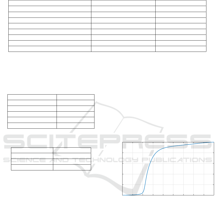
Table 1: Demographic Summaries for Active Smartphone Panelists and US Smartphone Users.

Demographic Active Smartphone Panelists US Smartphone Users

Mean Age (Years)

37.08 (12.54) 41.30 (15.08)

Gender (% Male) 26.42 50.08

Education (% w/ Some College or Less) 62.18 53.04

Marital Status (% Married) 41.45 48.96

Household Income (% <50K USD) 64.08 40.72

Mean Household Size 2.96 (1.51) 3.05 (1.61)

Mean Children in Household 0.91 (1.19) 0.74 (1.27)

Race (% White) 70.98 71.53

US smartphone user demographic data is from Pew Research survey (June-July 2015, subpop with smartphone n=1327) (Pew Internet and

American Life Project, 2015). The survey utilizes weighting to population parameters of census data to create nationally representative results

(refer to (Pew Research Center, 2016)). We note that Verto Analytics also performs its own national surveys, we utilize the Pew Research

survey only for brevity.

All mean values also include standard deviations.

Table 2: Number of active panelists for different platform-

device type combinations in panel.

Device Type Active Panelists

Smartphone (Android) 435

Smartphone (iOS) 127

Tablet (Android) 78

Tablet (iOS) 47

PC (Windows) 630

Table 3: Number of active panelists with both device types

in panel.

Device Types Active Panelists

Smartphone/Tablet 77

Smartphone/PC 269

Tablet/PC 52

a browser page simply automatically refreshes at a

speciﬁc interval. In other words, sessions that consist

mostly of highly periodic HTTP requests rather than

actual browsing behavior (which is typically bursty).

We can utilize periodicity detection to identify these

cases.

For a given session, a group of related periodic

HTTP requests should all target the same domain

(for example, auto-refresh of the same page), thus we

check for periodicity for each set of requests to the

same second level domain within a session. In other

words, if a session has 10 requests to Amazon.com

and 10 requests to Google.com, we check for period-

icity on these two sets separately. If we ﬁnd period-

icity we simply remove the requests from the session.

Thus the enforced timeout, which is applied after the

periodicity detection, can shorten the session.

In terms of the actual periodicity detection pro-

cedure, we ﬁrst estimate the power spectral density

(PSD) of each set of requests by the squared coefﬁ-

cients of the discrete Fourier transform of the signal.

We then classify a signal as periodic if 50% or more of

the total signal power is contained in the top 10% (in

terms of power) of frequencies. We select this 50%

level empirically through examination of the cumu-

lative distribution function (CDF) of the fraction of

power in the top 10% of frequencies of the PSDs. This

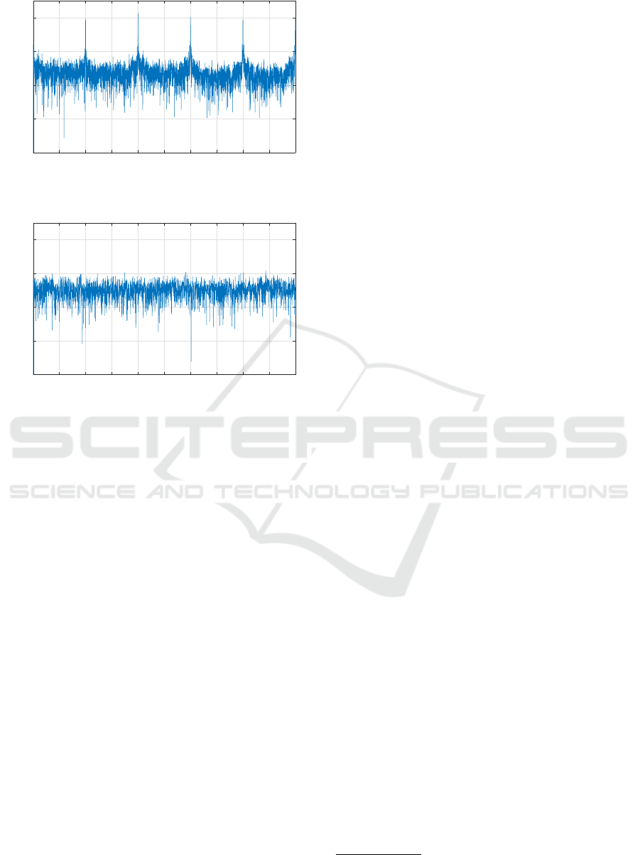
CDF is illustrated in ﬁgure 1. Furthermore, we illus-

trate the PSDs of two example request sets (from the

data): one periodic and one non-periodic in Figures 2

and 3 respectively.

Fraction of Power in Top 10% of Frequencies of PSDs

0.1 0.2 0.3 0.4 0.5 0.6 0.7 0.8 0.9 1

P (≤ x)

0.2

0.4

0.6

0.8

Figure 1: CDF for fraction of power in top 10% of frequen-

cies from power spectral densities.

We utilize this simple heuristic to detect signals

that are primarily periodic. This detection objective

contrasts with other methods that attempt to detect the

existence of any statistically signiﬁcant periodicity ir-

regardless of whether that periodicity dominates the

total power of the signal (as an example refer to (Vla-

chos et al., 2004)). In terms of the effects of both the

timeout and periodicity detection, the mean session

length of PC web browsing sessions is 15.1 min with-

out timeout or periodicity detection, 9.58 min with

only timeout, and 8.96 min with both timeout and pe-

riodicity detection.

Mobile Application Usage Concentration in a Multidevice World

Frequency (Hz)

0 0.05 0.1 0.15 0.2 0.25 0.3 0.35 0.4 0.45 0.5

Power

-10

-8

-6

-4

-2

Figure 2: Example power spectral density for set of HTTP

requests that are classiﬁed as periodic.

Frequency (Hz)

0 0.05 0.1 0.15 0.2 0.25 0.3 0.35 0.4 0.45 0.5

Power

-10

-8

-6

-4

-2

Figure 3: Example power spectral density for set of HTTP

requests that are classiﬁed as non-periodic.

5 RESULTS

We present the results of aggregate and individual

level app usage and concentration and then of corre-

lations of usage and concentration measures between

devices of the same user.

5.1 App Usage and Concentration

Statistics

5.1.1 Aggregate Level App Usage and

Distribution Fitting

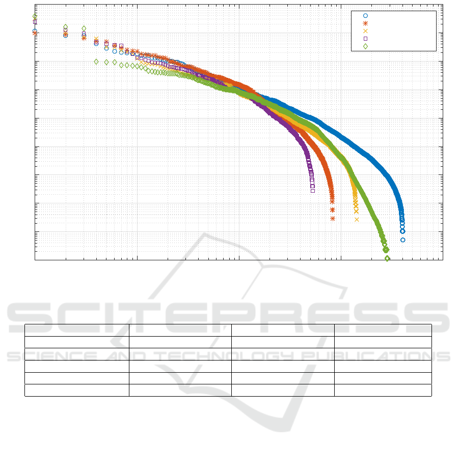
We ﬁrst examine the aggregate normalized app us-

age for different platform-device type combinations.

We illustrate these data through commonly used rank-

frequency distributions in Figure 4. Note that the

rank-frequency distribution is a transformation of the

discrete CDF that simply emphasizes a different part

of the data.

We ﬁnd that most of the distributions are concave

on a log-log scale with quickly decaying tails and sim-

ilar shapes. However, the PC distribution is a clear

outlier with a distinct shape and a large discontinuity

after the ﬁrst three apps. We ﬁnd that these ﬁrst three

apps are all web browsers and that these browsers ac-

count for about 66% of total PC app usage. Thus we

expect PC app usage to be very highly concentrated.

Interesting, the iOS distributions have much larger

values at the very ﬁrst rank and less overall ranks than

Android distributions. We ﬁnd that the large ﬁrst rank

is not a single app but instead a group of apps that

could not be identiﬁed by the iOS monitoring app due

to technical limitations. Furthermore, we ﬁnd that this

group of unidentiﬁable apps likely includes many in-

frequently utilized apps that would be seen at the tail

of the distribution, thus the group also accounts for the

fewer overall ranks. Hereafter, we remove this group

from the iOS data.

In terms of theoretical distribution ﬁts, the

shape of the data suggests a heavy tail distribu-

tion. Therefore we ﬁt several well known heavy

tail distributions (log-normal, exponential

, stretched-

exponential, power law, and truncated power law)

to the data through maximum likelihood estimations

(Alstott et al., 2014; Clauset et al., 2009). We utilize

a two step process for model selection: we ﬁrst select

a best ﬁt candidate via Akaike weights, we then per-

form Vuong likelihood ratio (LR) tests to ensure the

statistical signiﬁcance of the best ﬁt (Vuong, 1989)

compared to the other distributions.

We ﬁnd that log-normal distributions provide the

best ﬁts for the two smartphone and two tablet data

with both the highest Akaike weights and signiﬁ-

cantly (p ≤ 0.001) higher likelihoods than the other

distributions. Whereas a stretched exponential distri-

bution provides the best ﬁt for the PC data accord-

ing to the same criteria (p ≤ 0.001). The root mean

squared error (RMSE) of these best ﬁts in terms of

predicting the CDF are all less than 2%. We detail the

estimated best ﬁt parameters and RMSE of CDFs in

Table 4.

These log-normal and stretched exponential best

ﬁts clearly indicate that aggregate smartphone, tablet

or PC app usage do not follow a power law over the

entire data range. However we can ﬁnd the head pro-

portion (the proportion starting with the ﬁrst rank) of

each distribution that might follow a power law by

ﬁnding the optimal cut-off rank in terms of power

law ﬁtting (Alstott et al., 2014). We ﬁnd that for the

ﬁve distributions the cut-offs range from the 99th to

586th app rank and that even for the distribution with

the largest cut-off (iOS smartphone), the power law

would only cover 41% of the total ranks.

The exponential distribution is by deﬁnition not heavy

tailed but we included it for comprehensiveness.

WINSYS 2016 - International Conference on Wireless Networks and Mobile Systems

App Rank

Normalized App Usage

-9

-8

-7

-6

-5

-4

-3

-2

-1

Android Smartphone

Android Tablet

iOS Smartphone

iOS Tablet

Figure 4: Rank-frequency distributions of normalized app usage for device type-platform combinations.

Table 4: Parameter estimates and CDF error for aggregate app usage distribution ﬁtting.

Device Type Best Fit Distribution Parameter Estimates RMSE of CDF

(%)

Smartphone (Android) Log-Normal µ = 6.624 σ = 2.703 1.94

Smartphone (iOS) Log-Normal µ = 6.392 σ = 2.512 1.71

Tablet (Android) Log-Normal µ = 7.092 σ = 2.832 1.82

Tablet (iOS) Log-Normal µ = 6.381 σ = 2.481 1.41

PC (Windows) Stretched Exponential λ = 0.002 β = 0.173 1.78

Root mean squared error between empirical and predicted cumulative distribution functions.

5.1.2 Device Level App Usage and Distribution

Fitting

Next, we examine the device level app usage data. For

space considerations we limit our analysis and dis-

cussion to Android smartphones and PCs as we ﬁnd

the other platform-device type combinations are sim-

ilar, in terms of ﬁtting, to Android smartphones. We

perform distribution ﬁtting on the app usage data of

each Android smartphone and PC device with a simi-

lar method to Section 5.1.1.

For Android smartphones, we ﬁnd that 78% of de-

vices are best ﬁt by log-normal and 22% are best ﬁt by

stretched exponential according to Akaike weights.

Interestingly though not all of these best ﬁt candidates

are statistically signiﬁcant according to the LR tests.

For example, we ﬁnd that only 20% of devices are sig-

niﬁcantly (p ≤ 0.05) best ﬁt by log-normal. However

overall, we ﬁnd that 99% of devices are plausibly best

ﬁt by log-normal (in other words either log-normal is

the signiﬁcantly (p ≤ 0.05) best ﬁt or no other distri-

bution is a signiﬁcantly (p ≤ 0.05) better ﬁt).

We ﬁnd that the average RMSE of these plausible

best ﬁts in terms of predicting the CDF is 4%. Thus

the app usage of many smartphones can be accurately

ﬁt through a simple log-normal distribution. We illus-

trate the CDF of the app usage of an example Android

smartphone along with a log-normal best ﬁt in Figure

For PCs, we ﬁnd more variation in best ﬁts with no

single distribution covering a plurality of the devices

according to Akaike weights. This variation is likely

due to the relatively few apps and the dominance of

the web browser app on each PC.

5.1.3 Aggregate Level Concentration Statistics

We calculate the Gini coefﬁcient and Theil index for

Mobile Application Usage Concentration in a Multidevice World

App Usage (seconds)

P (≤ x)

0.2

0.4

0.6

0.8

Android Smartphone

Log-Normal

Figure 5: CDF of example Android smartphone app usage

and CDF of log-normal best ﬁt.

each aggregate platform-device type combination so

the concentrations can be studied and compared. We

also utilize a percentile-t bootstrap method (1000 iter-

ations) to calculate 95% conﬁdence intervals (CI) for

each concentration measure (Cowell and Flachaire,

2014). Importantly in our bootstrap method we utilize

individual devices (before aggregation) as the resam-

pling unit rather than the apps of the aggregate distri-

bution. The measures and CIs are detailed in Table

We make note of two important issues regarding

the comparison of concentration measures. First, in

the comparisons between two platform-device type

combinations (for example Android smartphone and

Android tablets) we do not account for users with a

device in each of the groups. In other words, the two

groups are not completely independent. However as

we will show in Section 5.2 there is almost no corre-

lation of Theil indexes between devices of the same

user. Therefore we ignore this dependence. Second,

percentile-t bootstrap CIs of inequality measures of

heavy tailed data can be suspect depending on the

heaviness of the tail (Cowell and Flachaire, 2014).

However they still provide signiﬁcant improvements

over pure asymptotic CIs, therefore we proceed with

caution

In general terms, we ﬁrst note that all device

types have relatively high app usage concentration as

shown by, for example, the Gini coefﬁcients and as

illustrated in the rank-frequency distributions. Previ-

ously, Jung et al. (2014) found that aggregate Android

smartphone app usage from a panel in Korea had a

Gini coefﬁcient of 0.74. Thus our Android smart-

phone Gini coefﬁcient of 0.96 suggests even higher

concentration. The difference might result from dif-

ferent panel time-frames or panelist cultural differ-

ences. Speciﬁcally the panel of Jung et al. (2014) was

We look to utilize more robust CI methods such as ﬁnite

mixture model CIs as detailed in Cowell and Flachaire

(2014) in future work.

a panel from Korea in November 2011 compared with

our panel from the United States in February 2015.

In terms of comparison between device types, we

ﬁnd that Android and iOS smartphones have sig-

niﬁcantly higher app usage concentrations than An-

droid and iOS tablets respectively (note the non-

overlapping CIs indicate at least p ≤ 0.05). These dif-

ferences can be partly explained through differences

in the primary types (categories) of apps utilized with

each device type. To illustrate this phenomenon we

ﬁrst calculate the aggregate normalized usage times

and Theil indexes for each app category for both An-

droid smartphone and tablets. We then plot these pairs

as a scatterplot for the two device types in Figure 6.

As illustrated, we ﬁnd that a larger fraction of

smartphone usage is from higher Theil index cate-

gories (like Social Networking) compared to tablets.

Similarly a larger fraction of tablet usage is from

lower Theil index categories (like Games and Kids).

Interestingly some categories (such as Uncategorized)

have both substantially different Theil indexes and

normalized usage between device types. These results

potentially indicate both inter and intra-category com-

ponents to the differences between aggregate smart-

phone and tablet concentration.

In terms of theory, the higher usage concentration

of social networking (communication) apps compared

to other categories such as games has also been doc-

umented by Jung et al. (2014). They suggest that the

difference is related to network effects wherein the

value of a communication service is proportional to

the number of users utilizing the service. Our anal-

ysis supports this supposition by illustrating that the

difference also exists on tablet devices and thus is not

device type speciﬁc.

In terms of platform differences, concentration

of iOS (smartphone and tablet) usage is not signiﬁ-

cantly different compared to concentration of Android

(smartphone and tablet) usage.

Finally, the signiﬁcantly (p ≤ 0.05) higher con-

centration of PC app usage than any other device type

is, as mentioned, due to the web browser as the dom-

inant app.

5.1.4 Device Level Concentration Statistics

In terms of the device level concentration, we calcu-

late the Gini coefﬁcient and Theil index for the app

usage data of each individual device. To illustrate de-

vice level diversity, we plot the CDFs of individual

Theil indexes for each platform-device type combina-

tion in Figure 7. The ﬁgure indicates signiﬁcant di-

versity in terms of individual usage concentration for

all device types.

WINSYS 2016 - International Conference on Wireless Networks and Mobile Systems

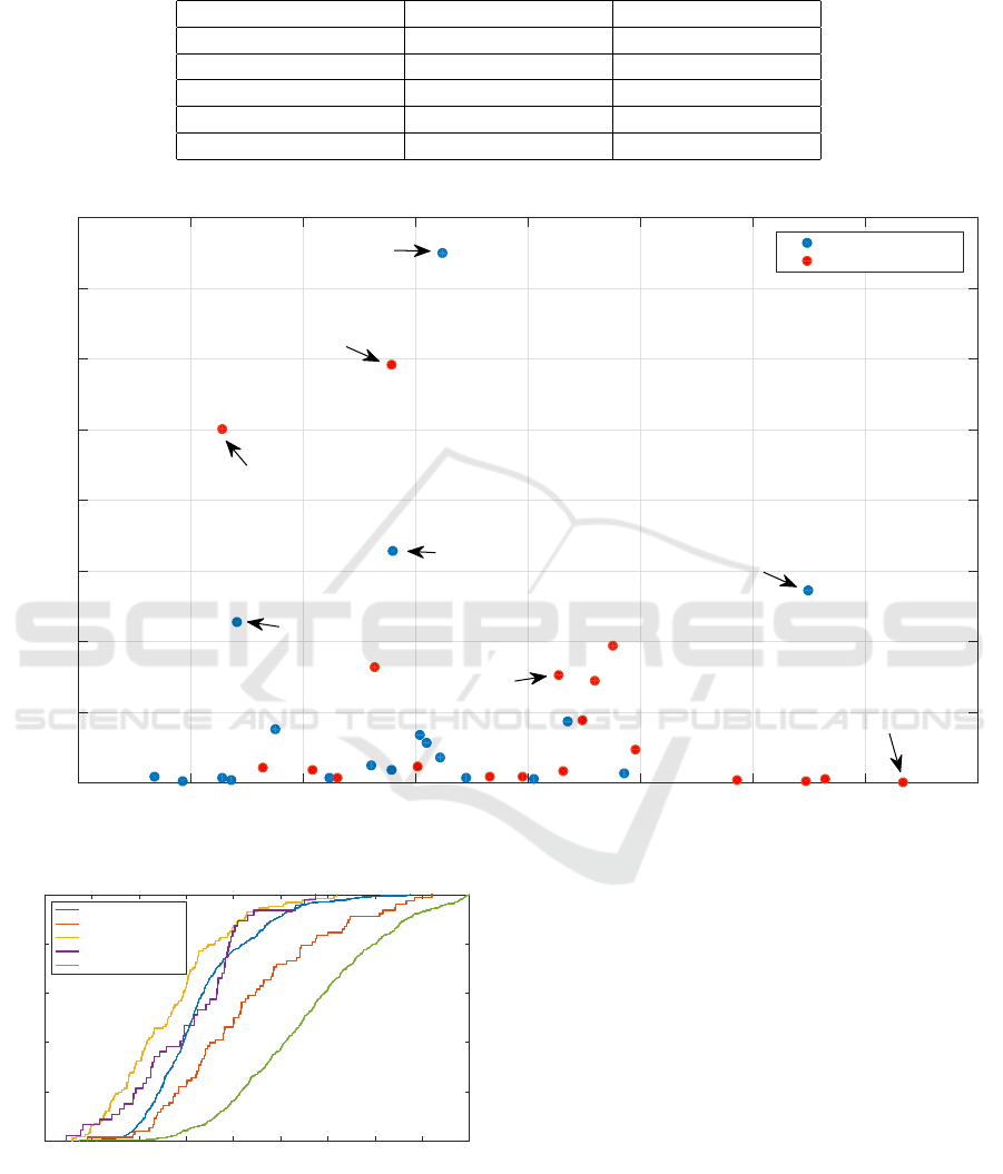
Table 5: Gini coefﬁcients and Theil indexes (including conﬁdence intervals

) for

aggregate data.

Device Type Gini Coefﬁcient Theil Index

Smartphone (Android) 0.962 [0.961, 0.968] 0.436 [0.433, 0.457]

Smartphone (iOS) 0.939 [0.935, 0.952] 0.425 [0.405, 0.462]

Tablet (Android) 0.920 [0.908, 0.935] 0.365 [0.333, 0.385]

Tablet (iOS) 0.904 [0.883, 0.930] 0.380 [0.329, 0.436]

PC (Windows) 0.976 [0.976, 0.981] 0.601 [0.595, 0.625]

95% conﬁdence intervals based on percentile-t bootstrap method.

Theil Index of Category For Device Type

0.2 0.3 0.4 0.5 0.6 0.7 0.8 0.9 1

Normalized App Usage (as Fraction of Total App Usage of Device Type)

0.05

0.1

0.15

0.2

0.25

0.3

0.35

0.4

Android Smartphone

Android Tablet

Social Networking

Utilities

Games and Kids

Uncategorized

Sports

Figure 6: Scatterplot of Normalized app usage vs. Theil indexes for app categories by device type (Android).

Theil Index

0.1 0.2 0.3 0.4 0.5 0.6 0.7 0.8 0.9 1

P (≤ x)

0.2

0.4

0.6

0.8

Android Smartphones

Android Tablets

iOS Smartphones

iOS Tablets

Figure 7: CDFs for device level Theil indexes for each

platform-device type combination.

Next, we compare the typical individual concen-

tration between device types. We calculate the me-

dian (with 95% CI) Gini coefﬁcient and Theil index

for each combination and detail these medians and

CIs in Table 6.

Interestingly, we ﬁnd that the median Theil index

of Android tablets is signiﬁcantly (p ≤ 0.05) larger

than that of Android smartphones. This contrasts with

our aggregate level analysis which found the opposite

phenomenon. Similarly, the platform comparison be-

tween Android and iOS smartphones also contrasts

with the aggregate level analysis. These differences

underscore the importance of analysis at both the ag-

gregate and individual level.

Though in terms of PCs we ﬁnd unsurprisingly

that the median Theil index of PC is signiﬁcantly

higher than all other device types. This in in line with

the aggregate level analysis.

Mobile Application Usage Concentration in a Multidevice World

Table 6: Median Gini coefﬁcients and Theil indexes (including conﬁdence intervals

)

for device level data.

Device Type Median Gini Coefﬁcient Median Theil Index

Smartphone (Android) 0.856 [0.850, 0.861] 0.415 [0.405, 0.423]

Smartphone (iOS) 0.807 [0.787, 0.818] 0.363 [0.322, 0.393]

Tablet (Android) 0.888 [0.857, 0.895] 0.507 [0.450, 0.551]

Tablet (iOS) 0.813 [0.789, 0.839] 0.417 [0.348, 0.468]

PC (Windows) 0.929 [0.923, 0.935] 0.651 [0.638, 0.669]

95% conﬁdence intervals based on binomial method.

5.2 Correlation of App Usage Measures

between a User’s Devices

Finally, we can also compare measures of app usage

for different devices of the same user. In this way we

can determine if app usage measures are correlated

across devices of the same user.

We examine two distinct measures: the Theil in-

dex and the total number of utilized apps. Further-

more, for each measure we compare three differ-

ent device type combinations: smartphone and tablet

(smartphone/tablet), smartphone and PC (smart-

phone/PC), and tablet and PC (tablet/PC). For each

statistic-device type combination (for example smart-

phone/PC Theil index) we calculate the Pearson cor-

relation coefﬁcient and the signiﬁcance level of the

coefﬁcient according to the related student’s t-test.

Table 7 details these coefﬁcients and signiﬁcance lev-

els.

In terms of Theil index, we ﬁnd that all combi-

nations are not signiﬁcant and near zero. Thus ex-

trapolation of app usage concentration from a single

device to other devices of the same user might be dif-

ﬁcult. The likely reason for the low correlation be-

tween the mobile devices and PC is again related to

web browsers as the dominant platform for apps on

PCs. Hence future work might try to include browser

based apps.

In terms of the total number of utilized apps, we

ﬁnd that the smartphone/tablet correlation is posi-

tive but not signiﬁcant, the tablet/PC correlation is

negative and signiﬁcant (p ≤ 0.05), and the smart-

phone/PC correlation is not signiﬁcant and near zero.

The signiﬁcant negative correlation of tablet/PC

might relate to device substitution between tablets and

PCs. In other words, users might perform tasks on

their tablets that they would otherwise perform on

their PCs. Therefore the more apps utilized on the

tablet, the less apps utilized on the PC. In general,

tablets and PCs are more often seen as substitutes

rather than smartphones and PCs because both tablets

and PCs are typically larger and less mobile (Xu et al.,

2015). To further support this theory, we calculate the

correlation between the total usage times (sum of all

app sessions) of tablet/PC. We also ﬁnd a signiﬁcant

(p ≤ 0.05) correlation of −0.242.

Similarly, the weak and non-signiﬁcant correla-

tion of smartphone/tablet might relate to device com-

plementation. In other words, users primarily perform

different types of tasks on smartphones and tablets.

Thus the number of utilized apps on smartphone and

tablet should be uncorrelated. Interestingly, we can

better understand app usage across smartphones and

tablets by examining the similarity between the smart-

phone app set and tablet app set of the same user.

Thus if smartphones and tablets are primarily compli-

mentary then the similarity should be relatively small.

For such an examination we need a measure to

deﬁne the similarity between the two app sets. We

utilize the well known Jaccard similarity coefﬁcient

which is simply the cardinality of the intersection of

two sets divided by the cardinality of the union of

those sets as detailed for sets A and B in Equation

J(A, B) =

|A ∩ B|

|A ∪ B|

(3)

We calculate the Jaccard similarity between the sets

of apps for each user with a smartphone and tablet

that share the same platform

We can then examine the distribution of the Jac-

card similarities of the 57 applicable users. We illus-

trate the distribution as a CDF plot in Figure 8. We

include the distribution of a random matching (per-

mutation) of the app sets in the plot for reference. We

ﬁnd users are quite evenly dispersed with similarities

between 5% and 25% but that no user has a simi-

larity larger than 25%. In other words no user uses

more than 25% of their total (utilized) smartphone

and tablet apps on both smartphone and tablet. This

supports our hypothesis of smartphone/tablet compli-

mentarity.

Finally, we can also test if the calculated user simi-

larities would be expected simply based on the overall

Again we note that application package names are plat-

form speciﬁc hence we cannot analyze users with smart-

phones and tablets with different platforms.

WINSYS 2016 - International Conference on Wireless Networks and Mobile Systems

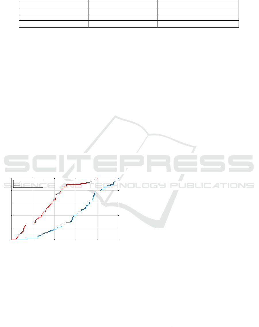
Table 7: Pearson correlation coefﬁcients (including signiﬁcance levels

) for Thiel indexes and total number

of utilized apps for different device type combinations.

Device Type Combination Correlation (Theil Index) Correlation (Number of Apps)

Smartphone/Tablet (n=77) 0.054 0.146

Smartphone/PC (n=269) 0.022 -0.024

Tablet/PC (n=52) 0.042 -0.305*

* : 5%, ** : 1%, *** : 0.1%

popularity of each app. In other words, is there any

statistically signiﬁcant similarity between the user’s

smartphone and tablet app sets?

For this test we utilize the median similarity as the

test measure for a permutation test. For the 57 users

this median similarity is 0.169. Speciﬁcally we per-

mute the smartphone and tablet app sets such that the

links between app sets of the same user are broken.

We then recalculate the median similarity over the 57

random matchings of smartphone and tablet app sets.

We repeat this entire permuting and recalculation pro-

cess for 100000 iterations to get a distribution of me-

dian similarities. We then ﬁnd the percentile values

corresponding to difference signiﬁcance levels.

The permutation test gives a 99.99% percentile

similarity of 0.104, thus suggesting that the empirical

similarity of 0.169 is highly signiﬁcant (p ≤ 0.0001).

Thus we do ﬁnd a statistically signiﬁcant similarity,

even though the maximum similarity of users is rela-

tively low.

Jaccard Similarity between Smartphone and Tablet App Sets

0 0.05 0.1 0.15 0.2 0.25

P (≤ x)

0.2

0.4

0.6

0.8

Users

Random Matching

Figure 8: CDF of users Jaccard similarities between their

smartphone and tablet app sets and CDF for a random

matching of smartphone and tablet app sets.

6 REPLICABILITY AND

GENERALIZABILITY

Generalizing or replicating a given panel based study

is typically difﬁcult in areas with rapid technological

and behavioral change such as mobile device usage.

Thus concerns about the usefulness of such studies

have been raised. Overall though, we take the view

that such panel based studies are primarily studies

about the panel populations themselves and that the

value lies in allowing researchers to contrast experi-

ences with diverse user populations to construct an

overall understanding of user diversity and behavior.

Thus our study provides an point of reference for fur-

ther multidevice studies. We refer to (Church et al.,

2015) for a thorough discussion on this topic.

7 DISCUSSION

In terms of applications, as mentioned, our research

has implications for understanding and modeling the

landscape of mobile advertising. For example, from

the ad demand side, our research suggests that total

app ad inventory and the concentration of that inven-

tory between certain apps depends strongly on app

category and device type. Whereas, similarly from the

ad supply side, our research suggests that apps in cer-

tain categories and device types might have more col-

lective bargaining power (against large ad exchanges

due to this concentration) than apps in other cate-

gories and device types

Furthermore such usage concentration research

will become more important as the mobile ad mar-

ket (speciﬁcally display ads) potentially shifts from

an impression (how many views) to impression time

(how many views and how long is each view) based

business model (see Rula et al. (2015) for further ex-

planation). This shift seems like a possibility given

the impact of impression time on ad recognition and

recall (Goldstein et al., 2011).

8 RELATED WORK

The related work can divided into previous studies

that have examined smartphone application usage and

previous studies that have included multiple device

types.

We note that not all apps utilize ads but that mobile ads

have become the dominant mobile app monitization strat-

egy.

Mobile Application Usage Concentration in a Multidevice World

8.1 Mobile Application Studies

ohmer et al. (2011) performed one of the ﬁrst large

scale study on mobile app usage with a panel of An-

droid smartphone users. They utilized a similar con-

cept of app sessions deﬁned by foregrounding and

backgrounding of apps. However they did not look

at the app usage concentration as their focus was

on sequential and temporal app patterns. Similarly

Soikkeli et al. (2013) analyzed smartphone app us-

age from a panel of Finnish smartphone users. They

detailed app usage statistics for several very popu-

lar apps but again do not look at usage concentration

among apps.

Falaki et al. (2010) analyzed smartphone app us-

age with two panels of users: one Windows Phone

and one Android based. They do illustrate and model

device-level app usage and ﬁnd that exponential dis-

tributions ﬁt most device app usage data well.

Closest to our work, Jung et al. (2014) examined

the aggregate app usage for a panel of Korean An-

droid smartphone users. They found highly concen-

trated usage though with lower Gini coefﬁcient than

the coefﬁcient for our smartphone data. They also

found differences in usage concentration between app

categories. However, they only examined aggregate

level app usage and did not examine device level app

usage. Furthermore, they did not examine app usage

concentration across multiple device types.

8.2 Multidevice Studies

Montanez et al. (2014) and Wang et al. (2013) exam-

ined multidevice usage but often only from the per-

spective of a single app (search) as the data was col-

lected from Microsoft’s search service (Bing).

Hintze et al. (2014) analyzed both smartphone and

tablet usage from the large Device Analyzer dataset.

Device Analyzer is a dataset based on a popular An-

droid device monitoring app from Cambridge Uni-

versity (Wagner et al., 2014). The dataset contains

both smartphone and tablet devices however corre-

lating usage of smartphone and tablet devices to a

single user is not possible thus comparing app us-

age between devices with the same user is infeasible.

Furthermore individual app names are not available

therefore app-speciﬁc insights are difﬁcult to extract.

Finally, Google (2012) and Microsoft (2013) stud-

ied multidevice usage through combinations of sur-

veys, user diaries, and device meters but did not study

multidevice app usage concentration.

9 CONCLUSIONS

In this work we have analyzed app usage with a fo-

cus on usage concentration in a multidevice context

including smartphones, tablets, and personal comput-

ers. Furthermore, we analyze usage concentration on

both an aggregate (market) level and individual device

level. Thus we provide a thorough view of app usage

concentration.

We highlight a few key takeaways from our analy-

sis. Overall, we show that, on an aggregate level, app

usage concentration will vary signiﬁcantly by device

type and thus future work, for example in modeling,

should take these differences into account to gain a

holistic view. Whereas, on an individual level, we ﬁnd

signiﬁcant diversity in app usage concentration even

for users with the same device type, therefore charac-

terizing a typical user is difﬁcult. Finally, we show

that several app usage measures are not strongly cor-

related between devices of the same user, thus empha-

sizing the need to capture all of users devices rather

than simply extrapolating from a single device. In

other words, a multidevice approach is warranted.

REFERENCES

Alstott, J., Bullmore, E., and Plenz, D. (2014). powerlaw:

A python package for analysis of heavy-tailed distri-

butions. PLoS ONE, 9(1):e85777.

ohmer, M., Hecht, B., Sch

oning, J., Kr

uger, A., and Bauer,

G. (2011). Falling asleep with angry birds, facebook

and kindle: A large scale study on mobile application

usage. In Proceedings of the 13th International Con-

ference on Human Computer Interaction with Mobile

Devices and Services, MobileHCI ’11, pages 47–56,

New York, NY, USA. ACM.

Church, K., Ferreira, D., Banovic, N., and Lyons, K. (2015).

Understanding the challenges of mobile phone usage

data. In Proceedings of the 17th International Con-

ference on Human-Computer Interaction with Mobile

Devices and Services, MobileHCI ’15, pages 504–

514, New York, NY, USA. ACM.

Clauset, A., Shalizi, C. R., and Newman, M. E. J. (2009).

Power-law distributions in empirical data. SIAM Re-

view, 51(4):661–703.

Cowell, F. A. and Flachaire, E. (2007). Income distribution

and inequality measurement: The problem of extreme

values. Journal of Econometrics, 141(2):1044–1072.

Cowell, F. A. and Flachaire, E. (2014). Statistical methods

for distributional analysis. In Atkinson, A. and Bour-

guignon, F., editors, Handbook of Income Distribution

SET vols. 2A-2B, Handbooks in economics. Elsevier

Science.

Falaki, H., Mahajan, R., Kandula, S., Lymberopoulos, D.,

Govindan, R., and Estrin, D. (2010). Diversity in

WINSYS 2016 - International Conference on Wireless Networks and Mobile Systems

smartphone usage. In Proceedings of the 8th In-

ternational Conference on Mobile Systems, Applica-

tions, and Services, MobiSys ’10, pages 179–194,

New York, NY, USA. ACM.

Goldstein, D. G., McAfee, R. P., and Suri, S. (2011). The

effects of exposure time on memory of display adver-

tisements. In Proceedings of the 12th ACM Confer-

ence on Electronic Commerce, EC ’11, pages 49–58.

Google (2012). The new multi-screen world: Un-

derstanding cross-platform consumer behavior.

https://think.withgoogle.com/databoard/media/pdfs/the-

new-multi-screen-world-study research-studies.pdf.

Hays, R. D., Liu, H., and Kapteyn, A. (2015). Use of in-

ternet panels to conduct surveys. Behavior Research

Methods, 47(3):685–690.

Hintze, D., Findling, R. D., Scholz, S., and Mayrhofer, R.

(2014). Mobile device usage characteristics: The ef-

fect of context and form factor on locked and unlocked

usage. In Proceedings of the 12th International Con-

ference on Advances in Mobile Computing and Multi-

media, MoMM ’14, pages 105–114. ACM.

Jung, J., Kim, Y., and Chan-Olmsted, S. (2014). Measuring

usage concentration of smartphone applications: Se-

lective repertoire in a marketplace of choices. Mobile

Media & Communication, 2(3):352–368.

Microsoft (2013). Cross-screen engagement.

http://advertising.microsoft.com/es-xl/WWDocs/

User/display/cl/researchreport/1932/global/Cross

reenWhitepaper.pdf.

Montanez, G. D., White, R. W., and Huang, X. (2014).

Cross-device search. In Proceedings of the 23rd ACM

International Conference on Conference on Informa-

tion and Knowledge Management, CIKM ’14, pages

1669–1678, New York, NY, USA. ACM.

Pew Internet and American Life Project (2015). June

10-july 12, 2015 gaming, jobs and broad-

band. http://www.pewinternet.org/datasets/june-10-

july-12-2015-gaming-jobs-and-broadband/.

Pew Research Center (2016). Our survey methodology in

detail. http://www.pewresearch.org/methodology/u-s-

survey-research/our-survey-methodology-in-detail/.

Roberto, E. (2015). The Boundaries of Spatial Inequal-

ity: Three Essays on the Measurement and Analysis

of Residential Segregation. PhD thesis, Yale Univer-

sity.

Rula, J. P., Jun, B., and Bustamante, F. (2015). Mobile

ad(d): Estimating mobile app session times for better

ads. In Proceedings of the 16th International Work-

shop on Mobile Computing Systems and Applications,

HotMobile ’15, pages 123–128.

Soikkeli, T., Karikoski, J., and Hammainen, H. (2013).

Characterizing smartphone usage: Diversity and end

user context. International Journal of Handheld Com-

puting Research, 4(1):15–36.

Theil, H. (1967). Economics and information theory.

Studies in mathematical and managerial economics.

North-Holland Pub. Co.

Vlachos, M., Meek, C., Vagena, Z., and Gunopulos, D.

(2004). Identifying similarities, periodicities and

bursts for online search queries. In Proceedings of

the 2004 ACM SIGMOD International Conference on

Management of Data, SIGMOD ’04, pages 131–142.

Vuong, Q. H. (1989). Likelihood ratio tests for model se-

lection and non-nested hypotheses. Econometrica,

57(2):307–333.

Wagner, D. T., Rice, A., and Beresford, A. R. (2014). De-

vice analyzer: Understanding smartphone usage. In

Mobile and Ubiquitous Systems: Computing, Net-

working, and Services, pages 195–208. Springer.

Wang, Y., Huang, X., and White, R. W. (2013). Charac-

terizing and supporting cross-device search tasks. In

Proceedings of the Sixth ACM International Confer-

ence on Web Search and Data Mining, WSDM ’13,

pages 707–716, New York, NY, USA. ACM.

Xu, K., Chan, J., Ghose, A., and Han, S. P. (2015). Bat-

tle of the channels: The impact of tablets on digital

commerce. Management Science.

Xu, Q., Erman, J., Gerber, A., Mao, Z., Pang, J., and

Venkataraman, S. (2011). Identifying diverse usage

behaviors of smartphone apps. In Proceedings of the

2011 ACM SIGCOMM Conference on Internet Mea-

surement Conference, IMC ’11, pages 329–344.

Mobile Application Usage Concentration in a Multidevice World