Facilitating Robotic Subtask Reuse by a New Representation of

Parametrized Solutions

Jacob P. Buch, Lars C. Sørensen, Dirk Kraft and Henrik G. Petersen

SDURobotics, The Maersk Mc-Kinney Moller Institute, University of Southern Denmark, Campusvej 55, Odense, Denmark

Keywords:

Industrial Assembly Automation, Uncertainty Handling, Dynamic Simulation, Reuse of Experimental Data.

Abstract:

In this paper, we suggest a coherent way of representing results from experiments associated with robotic

assembly. The purpose of the representation is to be able to reuse the experiments in other assembly settings.

A main novelty in our representation is the inclusion of ﬁne grained experimental uncertainties such as e.g.

deviations between a sensed object pose and the actual pose, and we discuss why it is very important for the

reusability of experiments to include these uncertainties. Under the reasonable assumption that we can repre-

sent the uncertainties as a region around the origin in a potentially high dimensional Cartesian space, we show

that we can efﬁciently represent the studied deviations by storing experiments on a so called spherical lattice.

We illustrate that the representation works by studying simulation experiments on two different industrial use

cases involving grasping an object and mounting an object on a ﬁxture.

1 INTRODUCTION

Within industrial production involving assembly,

there is an ever increasing demand for faster response

times, smaller batch sizes and a higher degree of vari-

ation. In addition, there is a similar demand for a

higher degree of automation in order to decrease cost

and increase efﬁciency and reliability. Traditionally,

assembly operations have mostly been automated by

means of large static mechanical machinery with high

throughput and relying heavily on strict repeatabil-

ity. However, such machinery is only cost effective

for very large batch sizes that are supposed to run for

several or many years and are thus becoming increas-

ingly infeasible for the above mentioned varying low

volume production. Therefore, industry needs solu-

tions that are cheap and easy to install and program

and also easy to reconﬁgure to a new task or between

different already programmed tasks.

The issue can be addressed by modularization ap-

proaches both on the mechanical and programming

side. In this paper, we will purely focus on modu-

lar programming concepts. Concerning the program-

ming issue, a common approach has been to divide

overall assembly tasks into a set of “subtasks”. The

idea is that solutions to subtasks can be developed for

one (the ﬁrst) application and reused by combining

them into other applications. We adopt a wide used

deﬁnition of a subtask as having a well deﬁned inter-

face in terms of a precondition for executing the sub-

task and a postcondition that the subtask is expected

to produce and that can be used as precondition for the

subsequent subtask. The pre- and postconditions are

mostly deﬁned at a symbolic level such as for exam-

ple “objectA-in-gripper” or “objectB-detected”. The

solution to the subtask is formalized as a parameter-

ized control where the parameters are typically op-

timized manually for the application where the sub-

task is used. Together with a framework for inserting

and sequencing the programmed subtasks, the over-

all complexity of solving a new task is strongly re-

duced by the modularization. The naming and precise

deﬁnition of the subtasks and associated parametrized

controls varies in the literature (see Section 2), but the

above formulation captures the essential idea of the

various approaches.

A potential problem with solving new tasks in

general and also with the above approach is that it can

be a slow and cumbersome process to derive the opti-

mal (or good enough) parameters for the control. The

reason for the difﬁculty is that there are small varia-

tions in the conditions for each execution of the task

due to e.g. small random displacements of the objects.

One might be able to reduce these variations mechan-

ically and rely on strict repeatability as in traditional

automation, but to reduce costs and setup times, it

would be desirable to be able to select control param-

eters that account for these variations. In the current

Buch, J., Sørensen, L., Kraft, D. and Petersen, H.

Facilitating Robotic Subtask Reuse by a New Representation of Parametrized Solutions.

DOI: 10.5220/0005964100370048

In Proceedings of the 13th International Conference on Informatics in Control, Automation and Robotics (ICINCO 2016) - Volume 2, pages 37-48

ISBN: 978-989-758-198-4

state, the programmer basically teaches the program

relying on a limited set of experiments using his com-

mon sense. There is no theoretical foundation for this

programming activity and there is no framework for

representing the generated results. Although the in-

formation (such as which control methods gave which

results) from the experiments may be valuable when

applying the subtask to other contexts, all this infor-

mation is typically lost. In simulations or in a labo-

ratory setting, information about the actual variation

in each execution may be made available, and hence

it would be desirable to derive a formulation that al-

lows storing information on the actual variations and

the outcome in a systematic and reusable way.

In this paper, we provide a theoretical formaliza-

tion of teach-in programming of tasks with variations

and provide a simple example that illustrates that so-

lutions to subtasks that are programmed based on a

teach-in procedure will typically rely on an insufﬁ-

cient set of experiments. We then suggest how to for-

mulate a representation of experiments when we have

ground truth knowledge of the variations that allows

stored results to be easily reusable between different

applications of the same subtask. This leads to the

choice of representing executions in a systematic way,

where we suggest to use a hyperspherical lattice (an

equidistant multidimensional directional grid) for the

variations. We then derive how such a lattice can be

used to predict the outcome when executing a subtask

with an arbitrary variation using interpolation tech-

niques.

Finally, we show how we can use the method to

quantitatively study the robustness of a given con-

trol to variations by an experimentally derived semi-

analytical expression for the region of variations in

which the execution will be successful. We study

and validate the formulation using simulations with

knowledge of variations of two different frequent sub-

tasks, namely a grasping task and a placing on ﬁxture

task.

The paper is organized as follows: In Section 2,

we review the state-of-the-art in more detail. In Sec-

tion 3, we present the basics of our approach in terms

of a mathematical formalization of executions of sub-

tasks. In Section 4, we augment this formalization so

that it becomes possible to reuse experimental results

associated with optimized subtask control. This leads

to the creation of a hyperspherical lattice in Section

5 for representing the impact of variations so that re-

sults can be reused between applications. In Section

6, we validate our concept based on the two different

subtask examples. Section 7 concludes the paper.

2 RELATED WORK

The idea of dividing a task into subtasks with well

deﬁned interfaces is not at all new as it has been

studied for decades in particular in the Artiﬁcial In-

telligence community. Early work on this was on

the purely symbolic side. A prominent example that

has inspired much of the early work is the so called

Stanford Research Institute Problem Solver (STRIPS)

planner (Fikes and Nilsson, 1971). The planner uses

proven components with well deﬁned interfaces that

can be combined to ﬁnd a path from an initial state to

a goal state. The exploitation of the concept in robotic

tasks has in recent years evolved. A good example

is the work by Huckaby and Christensen (Huckaby

and Christensen, 2012), (Huckaby et al., 2013) which

uses STRIPS for planning. Their representation of an

action allows to use a SysML (System Modeling Lan-

guage - an extension to UML) and a Planning Domain

Deﬁnition Language to reduce the overhead for the

planning of new processes. They call their subtasks

“skills” these can for example be grasping, sensing

or inserting. Another formulation of subtasks is pre-

sented in (Pedersen and Kr¨uger, 2015) as a combin-

able function block which is also called a skill. The

formulation also uses pre- and postconditions for au-

tomated sequencing. The parametrization is supposed

to be provided by the user as the studied cases are

rather simple.

Concerning our approach addressing reuse of ob-

tained knowledge for assembly, the work presented

in (Bjorkelund et al., 2011) is very relevant. Here, a

knowledge base is developed that supports the reuse

and examples within assembly are presented. How-

ever, the authors do not present a method for how

the reuse is supposed to take place in general, and in

particular also not how the variations should be in-

cluded in the knowledge base. In (Wahrburg et al.,

2015) a simpler subtask type is deﬁned which only

contains the needed components for control and co-

ordination of a robot without any responsibility for

interfaces and planning. The focus is on making the

subtasks reusable by deﬁning them as generic tem-

plates where any case speciﬁc part is extracted from

parameters. Other subtask formulations can be found

in e.g. (Bøgh et al., 2012), (Guerin et al., 2015).

The research on optimizing subtasks has mainly

focused on one speciﬁc instance of the subtask. Much

of this work is still carried out using a classical

teach-in approach. For grasping great effort has

been put into designing automated off-line grasp gen-

eration (Miller et al., 2003), (Vahrenkamp et al.,

2011), (Bohg et al., 2014), (Rytz et al., 2015) and

benchmarking of grasp solutions (Kim et al., 2013)

ICINCO 2016 - 13th International Conference on Informatics in Control, Automation and Robotics

(Bekiroglu et al., 2011). In this process, dynamic sim-

ulation has shown to be a valuabletool. Examples like

GraspIt (Miller and Allen, 2004) and OpenGrasp (Ul-

brich et al., 2011) are publicly available simulators

designed speciﬁcally for grasping.

A subtask where both teach-in and ofﬂine meth-

ods have been used for optimization is the peg-in-

hole type insertion. In (Stemmer et al., 2006), (Stem-

mer et al., 2007) and (Song et al., 2014) force con-

trol based assembly strategies are proposed. They use

force feedback from the robot to determine the state

of the assembly subtask. In (Chhatpar and Branicky,

2005) and (Kim et al., 2012) the authors approach the

problem by ﬁnding efﬁcient search algorithms for the

process and thereby the relative position uncertainty

is indirectly found. Ofﬂine optimization techniques

using dynamic simulation are heavily used in (Buch

et al., 2014) and (Sørensen et al., 2016). An inser-

tion trajectory is found by optimizing the relative tra-

jectory between the peg and hole objects so that the

available compliance can be optimally exploited.

3 MATHEMATICAL

REPRESENTATION OF

SUBTASKS WITH A FIXED

APPLICATION AND A FIXED

CONTROL

In this section, we ﬁrst present a formulation of the

execution of an arbitrary subtask as a deterministic

mathematical function that maps from the detailed

settings before the execution to the detailed settings

after the execution. In turn, we formulate a subtask

success criterion (chosen by the operator) as a binary

function on the settings after the execution. We then

show that deriving the control based on optimizing

the success probability (using the chosen success cri-

terion) will mostly require a very high number of exe-

cutions, which calls for a representation where execu-

tion results from teach-in of one subtask can be reused

for a similar subtask.

Consider a subtask as described in the introduc-

tion and recall that a subtask has a parametrized con-

trol function. When the parameters have been opti-

mized, we shall refer to a “programmed solution” to

the subtask. The subtask then comprise symbolic pre-

and post-conditions and an executable program. We

can view the programmed solution as a map f : X →

Y described by a known function y(x) = f(x,c(x)),

where x ∈ X is the expected input state and y(x) ∈ Y

is the expected state after the execution. We will as-

sume that all elements in X satisfy the precondition

of the programmed solution and that X and Y can be

represented as integrable subsets of (potentially high

dimensional) Euclidean spaces. The state sets X and

Y may thus contain ﬁne grained information such as

e.g. object poses and can have different dimensions.

The function c(x) denotes the programmed solution.

However, this representation is not sufﬁcient to

provide a deterministic description of a programmed

solution for the subtask when variations occur. To de-

rive a deterministic description, we should include a

true state, say x

True

in an individual execution. The

true state will typically deviate from the expected

state x and these deviations differ from execution to

execution. The true state could for example con-

tain the actual pose of an object as opposed to the

expected state which would contain the pose com-

puted from sensorial data. Similarly, the outcome

True

will deviate from the expected outcome y. As

the ﬂuctuations are unknown (otherwise they would

be the expected values), we should thus view a pro-

grammed solution as an unknown function y

True

,c(x)). Unfortunately, it is not possible to

derive this function in the real industrial setting as

both x

True

and y

True

will be unknown in these. We

make the basic assumption that x

True

contains the rel-

evant data for the outcome of the execution so that

the function f

True

,c(x)) is deterministic. Fur-

thermore, we make the reasonable assumption that

True

(x,c(x)) ≡ f(x,c(x)). In industrial settings, the

programmer therefore in practice deﬁnes a success

criterion for the execution, which can be measured.

Formally, we can write such a success criterion as a

set S

(x) ⊆ Y. Notice that although we do not y

True

we may know whether it is in S

. Consider for ex-

ample a grasping task where the state y

True

holds un-

known information of the actual pose of the object

relative to the gripper frame, but we can still measure

whether the grasp was successful.

Assume now for simplicity that the expected state

x and thus also y and S

are ﬁxed. The theoretical

success probability is then:

s =

ρ(x

True

|x)δ

( f

True

,c(x)))dx

True

(1)

where ρ(x

True

|x) is the probability density of true

states given that the expected (typically measured)

state was x and δ

True

) is one if y

True

∈ S

and

zero otherwise. This success probability can then be

estimated without knowledge of ρ(x

True

|x) by simply

repeating experiments with the programmed solution

c(x) enough times.

It should be noticed, that such a procedure to ob-

tain an accurate estimate of s will often require many

experiments. Therefore it is also difﬁcult or impos-

sible for the programmer to know if a programmed

Facilitating Robotic Subtask Reuse by a New Representation of Parametrized Solutions

solution has been selected that works as desired in the

long run. To see this, consider an example with ten

different possible sets of control parameters of which

nine has a success probability of 1 − 3ε and the last

has a success probability of 1 − ε where we assume

that ε is small. Assume that we do M independent ex-

periments with each set of control parameters. Using

the Poisson approximation, we obtain that we need

to carry out on the order M = 1/δ

experiments to

obtain a standard deviation that will enable us to de-

rive the optimal programmed solution with a reason-

able certainty. With δ = 1%, the operator thus need

to carry out around 10,000 experiments with each set

of control parameters to be reasonable certain that the

solution with the 99% success rather than 97% suc-

cess has been selected. A further and more practical

study on intelligent sampling methods for optimizing

control parameters can be found in (Sørensen et al.,

2016) where it also found that many experiments are

needed.

To resolve the problem of having to perform many

experiments, it would be desirable to ﬁnd out how we,

for an application of a subtask, can reuse the experi-

ments with the same type of subtask carried out in

different applications with different settings. An ob-

vious difﬁculty with reusing programmed solutions is

that there will be differences in the objects to be han-

dled (different materials, mass density distributions,

geometries etc.). This may be formally handled by a

parametrization of the experimental settings through

augmenting the set of expected states X. Unfortu-

nately, there are even when disregarding these differ-

ences a couple of drawbacks when seeking to reuse

the programmed solutions: i) The control was op-

timized with a ρ(x

True

|x) associated with the given

experimental settings. In other applications, where

the programmed solution is to be used, the function

ρ(x

True

|x) may be signiﬁcantly different and thus the

control c(x) may be far from optimal. A good exam-

ple is grasping of a pose estimated object. The object

may be picked from a table with small variations in

height and tilt or from a bin with similar variations

in all pose dimensions. ii) In some experiments, it

may be difﬁcult to associate a reusable success region

. A good example is again grasping, where the suc-

cess region S

for a precision grasp strongly depends

on the accuracy requirements of the subsequent op-

eration. Hence, a traditionally programmed solution

(using e.g. one of the skill libraries mentioned in the

related work section) is only useful for reuse if the

changes in ρ(x

True

|x) and S

are negligible. In the

next section, we will devise a representation that al-

low signiﬁcant changes in ρ(x

True

|x) and S

and thus

substantially increase reusability.

4 AUGMENTED SUBTASK

REPRESENTATIONS FOR

REUSABILITY

In this section, we augment the representation of sub-

task executions so that they include the true states.

Clearly, the true states will not be available in the

real industrial settings, but this formulation opens for

the possibility of exploiting experiments performed in

laboratory conditions with sensors to obtain ground

truth information or (as we do in this paper) exploit-

ing experiments carried out in computer simulations

where all information of course is available. We dis-

cuss how to choose the represention and different

methods for storing the results of the executions both

in laboratory conditions and with computer simula-

tions.

To deal with different ρ(x

True

|x)’s and S

’s, we

need to devise a representation that is independent of

these. The most direct way of achieving that is to

simply study the propagation of true states relative to

the expected state in a coherent way.

If we describe the propagation of true states

True

= f

True

,c(x)) as y + e

= f

True

(x +

,c(x)), we may study the map as a propagation of

errors to the expected state e

= φ(e

,c(x),x) where

∈ E

and E

are small regions lo-

cated around the origin in the corresponding Eu-

clidean spaces belonging to X and Y. Notice that we

assume that the map φ(e

,c(x),x) is continuous in e

within the region E

. This is a reasonable assumption

since we are studying potentially successful actions.

We wish to derive a method that based on already per-

formed experiments is capable of predicting the out-

come of executing the programmed solution with an

arbitrary error e

without having to perform the exper-

iment with e

. In the simplest setting, we would wish

to be able to predict whether the experiment would

be successful, i.e. that f(x + e

,c(x)) ∈ S

. A fur-

ther step would be to be able to predict the value of

φ(e

,c(x),x). Here, we discuss two approaches that

could be taken

• Random sampling in E

together with a smooth-

ing technique such as e.g. Kernel Density Estima-

tion

• Interpolation in E

using a grid (e.g. based on a

hyperspherical lattice)

There are advantages and disadvantages with both ap-

proaches. The problem with random sampling is in

the search phase. If the dimension of E

is high,

the total number of samples needed will also be high,

and there would be a large overhead in ﬁnding the

neighbors that are needed in the Kernel Density based

ICINCO 2016 - 13th International Conference on Informatics in Control, Automation and Robotics

interpolation. The disadvantage with a spherical lat-

tice is that it requires that we can select the errors e

However, as we will deploy simulation for the exper-

iments, the selection problem does not occur and we

therefore choose the lattice approach. Hence, we will

devise a spherical lattice that will allow instantaneous

ﬁnding of the nearest lattice vectors for a given error

and how these can be used to predict the error propa-

gation e

= φ(e

,c(x),x).

5 CONSTRUCTION OF A

SPHERICAL LATTICE

In this section, we present an algorithm for construct-

ing a hyperspherical lattice where we adopt a method

from the literature and outline how it works. A spher-

ical lattice on a K-dimensional sphere is an organized

set of approximately equidistant points on the sphere.

In two dimensions these can be generated optimally

by simply tesselating the unit circle into N points with

angles 2πj/N for j = 1, ...,N. Already in three di-

mensions, there are no general optimal solutions al-

though there are special cases such as the icosahedral

distribution. In higher dimensions, it become even

more complicated, but several rather different meth-

ods for computing suitable lattices can be found in

the literature. Here we adopt the method from (Lovi-

solo and da Silva, 2001) as it has the advantage of

providing a lattice set that facilitates searching and

also allows the user to control the grid size rather pre-

cisely. For completeness, we state the algorithm here.

We ﬁrst deﬁne spherical coordinates for vectors in K

dimensions. If we write an arbitrary unit vector as

u = (u

,...,u

), a set of corresponding spherical co-

ordinates θ

,...,θ

K−1

can be deﬁned as:

= cosθ

k−1

j=1

sinθ

k = 1...K − 1 (2)

= Π

K−1

j=1

sinθ

(3)

The user then chooses an approximate distance be-

tween neighboring lattice vectors δ and a set can then

be found as follows. Choose ﬁrst ∆θ

= δ and per-

form the tesselation θ

)

= i

∆θ

. Assume now that a

tesselation has been derived for spherical coordinate

k − 1 and consider an arbitrary point of that tessela-

tion (θ

)

,θ

)

,...,θ

k−1

)

k−1

. We can then compute the

size of the tesselation of the spherical coordinate k by

computing:

∆θ

k−1

j=1

sinθ

)

(4)

and subsequently choose θ

)

= i

∆θ

. Notice that

for k > 1, we thus have a variable ∆θ

selected so that

the distance between adjacent points will be δ. Due

to boundaries on the spherical coordinate, the lattice

will not be perfect, but we have tested it to be useful

even for a rather small size of the lattice. Moreover,

the choice of δ should be rather intuitive for the user.

6 USING THE SPHERICAL

LATTICE TO APPROXIMATE

THE ERROR

TRANSFORMATIONS AND

SUCCESS REGIONS USING

SIMULATIONS

We now study a subtask using simulation. For any

input error e

, the simulator thus produces a resulting

error e

= φ(e

,c(x),x), and we wish to estimate this

map using our spherical lattice.

Lattice Data Generation: The ﬁrst step is to

choose an appropriate scaling (choice of unit) for each

of the coordinates of e

so that we can select the same

maximal error distance D for all directions (and thus

for all lattice vectors) that we wish to sample. For

each lattice vector, say u

, we select a tesselation ε

of error points along the vector u

where we perform

simulations. The next step is thus to perform simula-

tions with errors s

= iεu

for each lattice vector and

for i = 1, ... , ⌈

⌉. We record the deterministic out-

comes σ

= φ(s

,c(x)) generated by executing the

simulation.

Prediction: Consider now an arbitrary error e

We then search for the K nearest lattice vectors that

correspond to the corners in the K − 1 dimensional

hyperplane on the surface of the unit sphere to which

belongs. To do this efﬁciently, we may compute the

spherical coordinates of e

and use the structure of the

lattice to obtain the hyperplane with a rather limited

search. We then select the nearest tesselation point

relative to the size of e

and perform a weighted linear

interpolation between these to obtain an estimate of

φ(e

,c(x),x).

We are thus immediately able to use this for var-

ious studies such as to estimate the overall success

probability of the programmed solution c(x) for any

ρ(x

True

|x) and any S

by noticing that we can write

(1) as:

s =

ρ(x+ e

|x)δ

( f

True

(x+ e

,c(x)))de

(5)

and deploying a classical sample point based numeri-

cal integration schemes.

In this paper, we wish to illustrate the validity of

our method in a simple way by studying the success

Facilitating Robotic Subtask Reuse by a New Representation of Parametrized Solutions

regions directly. To determine the success region, we

for each lattice vector, say u

, compute the largest dis-

tance d

where all errors αu

belong to the success re-

gion when α ≤ d

. If all values up to Du

belongs to

the success region, we set d

= D.

For an arbitrary error vector e

, we then again

search for the K nearest lattice vectors that corre-

sponds to the corners in the K − 1 dimensional hy-

perplane on the surface of the unit sphere to which e

belongs. We can then provide a conservative estimate

by testing if e

is closer to the origin than the scaled

hyperplane with corners d

for the relevant K − 1

lattice vectors.

7 VALIDATING OUR CONCEPTS

ON TWO SUBTASKS

In this section, we test our concept on two subtasks.

The ﬁrst subtask consist of grasping of an industrial

object using a Robotiq two ﬁngered hand and the sec-

ond case is the placement of the same object into a ﬁx-

ture. For each subtask, three types of errors and asso-

ciated success regions are studied where each handles

a speciﬁc type of uncertainty. The ﬁrst error type in-

cludes the positional uncertainties of an object placed

on a table. The second includes errors in all three

positional dimensions to illustrate the concept for any

positional uncertainties. Lastly, a full six-dimensional

error illustrates any transformational uncertainty for

an object.

For each of the cases, we compare the actual out-

come (success/failure) with the predicted outcome

computed as outlined in the end of the previous sec-

tion. By this, we will study the value of using the

derived representation for a detailed robustness of a

given control to uncertainties.

7.1 Grasping of Industrial Object

Subtask

In the grasping subtask, an industrial part is grasped

by a Robotiq two ﬁngered gripper. The length of

the industrial part is 5cm and has a diameter of 3cm

where it is largest. The scene is shown in Figure 1.

The grasping strategy starts by the hand being placed

10cm above the graspinglocation and it is then moved

linearly down to the grasping location. At this posi-

tion, the gripper is set to close, and ﬁnally, the hand

is again lifted to the initial position. At this point, the

simulation is evaluated. In the evaluation, it is tested

whether the object is still in contact with both the ﬁn-

gers. If so, the action is evaluated as a success and

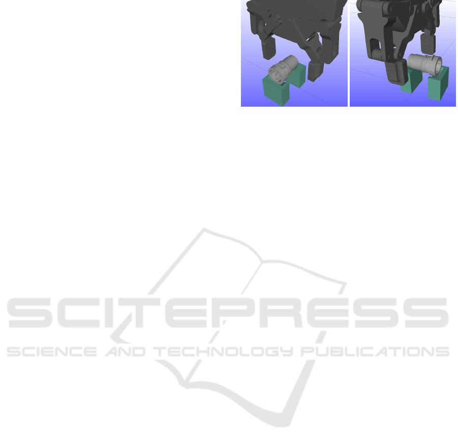
Figure 1: Scene for the grasping subtask. It consists of a

ﬁxed ﬁxture, a dynamic industrial object and a kinemati-

cally controlled Robotiq hand with dynamically controlled

ﬁngers.

otherwise as a failure.

The dynamic simulation engine chosen for this

task is the Open Dynamics Engine (Drumwright

et al., 2010), which is a widely used engine in the

robot community and has in particular been used

for grasping. The engine is interfaced using Rob-

Work(Ellekilde and Jorgensen, 2010). In the engine,

the friction between the ﬁngers and the industrial ob-

ject was set to µ = 0.9. The robotic hand was modeled

as individual bodies for each ﬁnger part connected by

joints. The ﬁnger is then driven by a torque added

between the base and the ﬁrst outermost ﬁnger part

which is used to pull the ﬁngers together when grasp-

ing the object. The object is picked from a simple ﬁx-

ture comprised of a box with a small cut out to hold

it in place. Contacts between ﬁxture and gripper are

ignored in simulation.

7.1.1 2D Positional Errors when Grasping

Objects from a Table

The industrial part is, in this case, perturbed in the di-

rections of a plane to simulate the errors which could

occur if the object was placed on a table, i.e. e

∈ R

The area is estimated by two different sets of lattice

vectors with respectively six and twelve vectors. The

search vector is maximally evaluated up to D = 12cm

and the used tesselation is ε = 1mm. The success ar-

eas are illustrated in Figure 2, together with 4000 ran-

dom perturbations generated from a realistic distribu-

tion. The distribution chosen was a two-dimensional

normal distribution with mean 0cm and standard de-

viation σ = 8cm in both directions and with no cor-

relation. Qualitatively, the plot shows that the region

is very well captured with these two rather sparse lat-

tices. Typically, the success area will grow in size

when reﬁning the lattice as the polyhedral shortcuts

will be smaller, which can also be seen in the Figure.

However, in the ﬁrst quadrant, the success area of the

12 lattice vector case is smaller than the 6 lattice case

ICINCO 2016 - 13th International Conference on Informatics in Control, Automation and Robotics

●

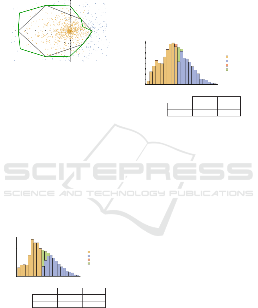
- 0.06 - 0.04 - 0.02 0.02 0.04

[m]

- 0.04

- 0.02

0.02

0.04

[m]

Figure 2: 2D success areas of the grasping action and 4000

perturbations taken from a two dimensional normal distri-

bution with mean 0 cm and standard deviation 9 cm in both

dimensions. Blue dots indicate a failure while yellow ind-

cate a success. The six search vector based success area is

illustrated in black and the twelve search vector based suc-

cess area is illustrated in green.

due to what seems to be a simulation artifact.

For quantiﬁcation, the performance is for all our

experiments measured with a confusion matrix and a

histogram. The histogram shows the distribution of

the four results from the confusion matrix with re-

spect to the distance to the boundary of the estimated

success region. Points inside the region have negative

distances in the histogram.

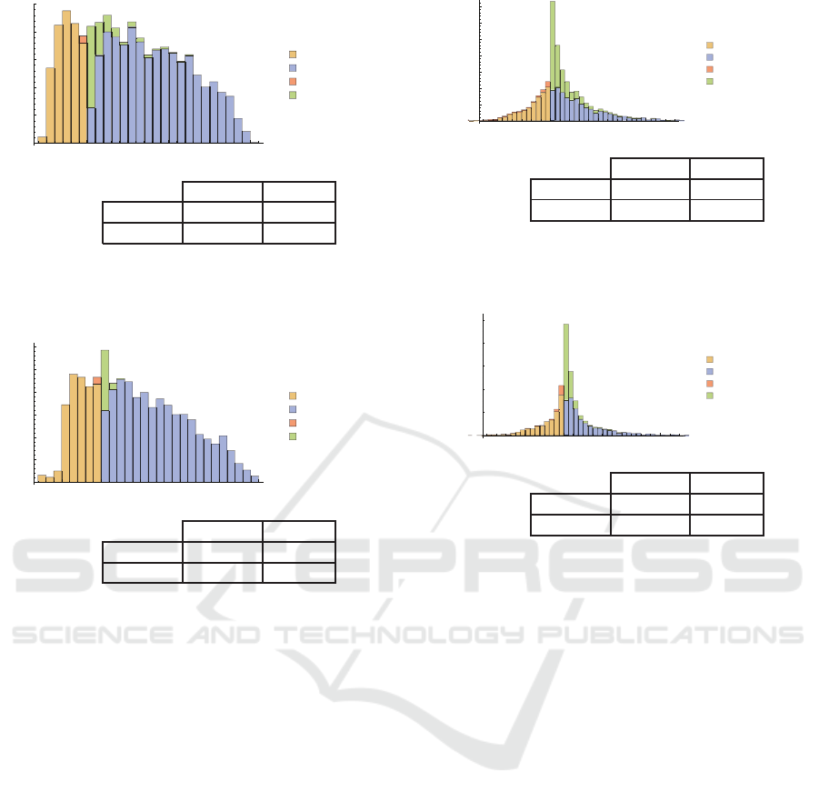
For the 2D case, the results are illustrated for the

coarse lattice with six vectors in Figure 3. The con-

fusion matrix illustrates a very good estimation where

92% of the experiments were correctly estimated with

respect to the success area and only 0.57% are a crit-

ical false positive. False positives are more critical

since they can result in unexpected failures whereas

false negatives just represent a too strict success area.

Notice also from the histogram that all of the false

estimates are close to the edge of the success area.

-0.04 -0.02 0.00 0.02 0.04 0.06

[m]

100

200

300

400

True Positive

True Negative

False Positive

False Negative

Predicted

Success Failure Total

Executed in Success 2111 305 2416

simulation Failure 9 1575 1584

Total 2120 1880 4000

Figure 3: Histogram and confusion matrix for the 2D po-

sitional errors based on six lattice vectors for the grasping

subtask.

For the twelve vectors based success area, the re-

sults are shown in Figure 4. Despite the artifact in

the ﬁrst quadrant, this success area has a better cover-

age of the real success area where 96% of all pertur-

bations were correctly estimated. It has as expected

a small increase to 1.5% in the critical false-positive

percentage due to the more tight estimation of the suc-

cess region.

-0.04 -0.02 0.00 0.02 0.04 0.06

[m]

100

150

200

250

300

350

True Positive

True Negative

False Positive

False Negative

Predicted

Success Failure Total

Executed in Success 2283 133 2416

simulation Failure 24 1560 1584

Total 2307 1693 4000

Figure 4: Histogram and confusion matrix for the 2D posi-

tional errors based on twelve lattice vectors for the grasping

subtask.

7.1.2 3D Positional Errors when Grasping an

Object

In the second experiment, we also include the third

positional dimension, i.e. e

∈ R

. To estimate the

success area, we again consider two lattices based re-

spectively on 12 and 42 vectors. As it is difﬁcult to

illustrate plots of the regions in more than two dimen-

sions, we have chosen to omit these. The performance

can howeveragain be estimated by a confusion matrix

and a histogram. We again used 4000 perturbations,

but nowtaken from a three-dimensional normal distri-

bution with identical standard deviationof σ = 8cm in

each dimension. The results with twelve lattice vec-

tors are shown in Figure 5.

The performance is not quite as good as for the

two-dimensional success area, but still more than 90%

are correctly estimated and still only less than 2% of

the critical false positive are present in both cases.

The performance for the success region based on 42

vectors is shown in Figure 6. The results in the con-

fusion matrix has again an increase in false positives

due to the tighter ﬁt, but has a larger decrease in false

negatives and thus an overall better representation of

the success region.

7.1.3 6D Errors for Grasping an Object

We now consider grasping objects with pose errors

in all six dimensions (three in position and three in

orientation). A success area is best represented by

Facilitating Robotic Subtask Reuse by a New Representation of Parametrized Solutions

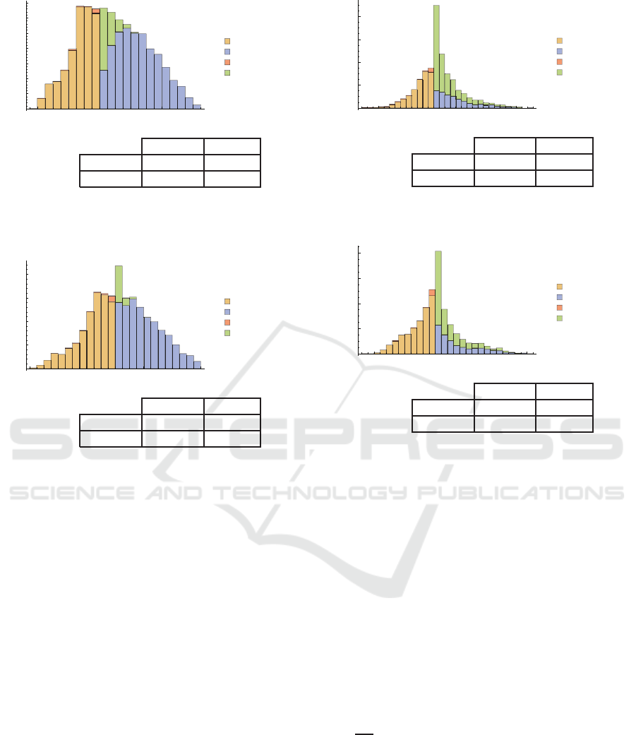
-0.04 -0.02 0.00 0.02 0.04 0.06

[m]

100

150

200

250

300

350

True Positive

True Negative

False Positive

False Negative

Predicted

Success Failure Total

Executed in Success 1515 370 1885

simulation Failure 26 2089 2115

Total 1541 2459 4000

Figure 5: Histogram and confusion matrix for the 3D po-

sitional errors based on 12 lattice vectors for the grasping

subtask.

-0.04 -0.02 0.00 0.02 0.04 0.06

[m]

100

200

300

400

True Positive

True Negative

False Positive

False Negative

Predicted

Success Failure Total

Executed in Success 1689 196 1885

simulation Failure 42 2073 2115

Total 1731 2269 4000

Figure 6: Histogram and confusion matrix for the 3D po-

sitional errors based on 42 lattice vectors for the grasping

subtask.

the lattice vectors if there is an equivalence between

translation and rotation. To ensure this, we have cho-

sen a relation of the units to be so that 1cm is equiv-

alent to 0.3rad roughly corresponding to an object of

a size of 5− 10cm. The success region is estimated

with lattices of respectively respectively 98 and 1004

lattice vectors corresponding to δ = 0.8 and δ = 0.5.

The performance is again studied using 4000 pertur-

bations, which is now taken from a distribution with

a standard deviation of 5cm in the three positional di-

mensions and σ = 1rad in roll, pitch and yaw.

The results for the success region estimated from

98 search vectors is illustrated in Figure 7. There is a

now a rather signiﬁcant set of 43.75 % of the actually

successful perturbations that are falsely predicted as

a false negative. This indicates that the conservative

success region estimate obtained from cutting off with

the polyhedral shortcuts now has an impact.

The results with 1004 lattice vectors are illustrated

in Figure 8. We see that the estimate is improved over

the 98 based six-dimensional success area, but there

are still many successful tests that were predicted as

-0.02 -0.01 0.00 0.01 0.02 0.03

[m]

200

400

600

800

True Positive

True Negative

False Positive

False Negative

Predicted

Success Failure Total

Executed in Success 1333 1750 3083

simulation Failure 68 849 917

Total 1401 2599 4000

Figure 7: Histogram and confusion matrix for the 6D errors

based on 98 lattice vectors for the grasping subtask.

-0.02 -0.01 0.00 0.01 0.02 0.03

[m]

200

400

600

800

True Positive

True Negative

False Positive

False Negative

Predicted

Success Failure Total

Executed in Success 1811 1272 3083

simulation Failure 64 853 917

Total 1875 2125 4000

Figure 8: Histogram and confusion matrix for the 6D errors

based on 1004 lattice vectors for the grasping subtask.

failure. For both cases, we however observe around 7

% of the failures were now false positives.

7.2 Placing in Fixture Subtask

The second investigated subtask is a placement of the

same industrial part into a ﬁxture. The scene is shown

in Figure 9 and consist of two elements. A compliant

ﬁxture and an industrial part which is kinematically

controlled. The compliance in the ﬁxture is modeled

by ﬁxing the body to the world with a damped spring.

The spring has a directional compliance which is set

to 0.0005m/N, the rotational compliance is set to

0.1

N·m

and the friction is chosen so the system is crit-

ically damped. The control used with the insertion

to simply place the object linearly from above. The

industrial object is initially held 15cm above the tar-

geted ﬁnal position in the ﬁxture. From that position,

the object is moved directly downwards to the ﬁnal

position. The simulation is then evaluated at simula-

tion end time. For evaluation, we examine the tip of

the ﬁxture. If the tip of the ﬁxture is at least 1cm in-

side the industrial part the simulation is evaluated as

ICINCO 2016 - 13th International Conference on Informatics in Control, Automation and Robotics

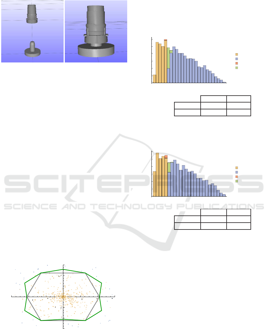
Figure 9: Scene for the place in ﬁxture case. The left im-

age shows the initial position and the right image the goal

position of the subtask.

a success, otherwise it is a failure.

Since this action is a tight ﬁt insertion, we found

based on recent studies (Thulesen and Petersen, 2016)

that ODE was not suitable to simulate the task. Based

on these studies, anonomous was chosen to accurately

simulate tight-ﬁt assembly. We used the standard set-

tings of the engine except for the friction coefﬁcient,

which was set to 0.4 corresponding to interactions be-

tween two plastic objects. We again study 2D and

3D positional errors and the 6D general error with the

same lattices as for the grasping subtask.

7.2.1 2D Positional Errors for Placing an Object

on a Fixture

The results for the estimation of the success region

were again obtained with 4000 perturbations and a

plot is shown in Figure 10. The perturbations are here

again taken from a two-dimensional normal distribu-

tion but with a lower standard deviation σ = 2.5cm

since this action is much less resilient to uncertain-

ties.

The quantitative results are again shown with con-

fusion matrices and histograms and are illustrated in

●

- 0.006 - 0.004 - 0.002 0.002 0.004 0.006

[m]

- 0.006

- 0.004

- 0.002

0.002

0.004

0.006

[m]

Figure 10: 2D success areas of the place in ﬁxture ac-

tion and 4000 perturbations taken from a two dimensional

normal distribution with mean 0cm and standard deviation

2.5cm in both dimensions. Blue dots indicate a failure

while yellow indcate a success. The six search vector based

success area is illustrated in black and the twelve search

vector based success area is illustrated in green.

Figure 11 and Figure 12 respectively. The results

show that both success regions are very well esti-

mated with only a few false classiﬁcations and the

performance looks very similar to the corresponding

results from the grasping action.

0.000 0.005 0.010 0.015 0.020

[m]

100

150

200

250

300

True Positive

True Negative

False Positive

False Negative

Predicted

Success Failure Total

Executed in Success 1143 161 1304

simulation Failure 7 2689 2696

Total 1150 2850 4000

Figure 11: Histogram and confusion matrix of 2D success

area estimated based on six search vectors for the place in

ﬁxture subtask.

0.000 0.005 0.010 0.015 0.020

[m]

100

150

200

250

300

True Positive

True Negative

False Positive

False Negative

Predicted

Success Failure Total

Executed in Success 1238 68 1306

simulation Failure 18 2676 2694

Total 1256 2744 4000

Figure 12: Histogram and confusion matrix of 2D success

area estimated based on twelve search vectors for the place

in ﬁxture subtask.

7.2.2 3D Positional Errors for Placing an Object

on a Fixture

This study is similar to the study for the success re-

gion for the three-dimensional grasping case, but with

the perturbations are taken from a distribution with

standard deviation of σ = 2.5cm in all three dimen-

sions. The results is shown in Figure 13 and Figure

14.

Again the quality of matching is similar to the

grasping subtask with only around 0.5% false pos-

itives, but here there is a somewhat surprising im-

provementon the false negativesby going to 42 lattice

vectors.

Facilitating Robotic Subtask Reuse by a New Representation of Parametrized Solutions

0.000 0.005 0.010 0.015 0.020

[m]

100

150

200

250

True Positive

True Negative

False Positive

False Negative

Predicted

Success Failure Total

Executed in Success 991 286 1276

simulation Failure 13 2710 2723

Total 1004 2996 4000

Figure 13: Histogram and confusion matrix of 3D success

area estimated based on twelve search vectors for the place

in ﬁxture subtask.

-0.005 0.000 0.005 0.010 0.015 0.020

[m]

100

150

200

250

300

True Positive

True Negative

False Positive

False Negative

Predicted

Success Failure Total

Executed in Success 1127 150 1277

simulation Failure 15 2708 2723

Total 1142 2858 4000

Figure 14: Histogram and confusion matrix of 3D success

area estimated based on 42 search vectors for the place in

ﬁxture subtask.

7.2.3 6D Errors for Placing an Object on a

Fixture

For this subtask, the last experiments also considers

all six dimensions of pose errors. The perturbations

are taken from a distribution with standard deviation

of σ = 2cm in the position and σ = 0.6rad in roll,

pitch and yaw. The performance of the success area

is shown in Figure 15 and Figure 16 for the success

area created from 98 search vectors and 1004 search

vectors respectively. Again, we obtain results that are

quite similar to those for the grasping subtask with

around 7% false positives.

8 CONCLUSION

In this paper, we have outlined how to represent out-

comes of experiments when uncertainties are avail-

able to be used in frameworks where robotic tasks are

divided into subtask components that are aimed at be-

-0.005 0.000 0.005 0.010

[m]

100

200

300

400

500

600

700

True Positive

True Negative

False Positive

False Negative

Predicted

Success Failure Total

Executed in Success 979 1275 2254

simulation Failure 116 1630 1746

Total 1095 2905 4000

Figure 15: Histogram and confusion matrix for the 6D er-

rors based on 98 lattice vectors for the place in ﬁxture sub-

task.

-0.005 0.000 0.005 0.010

[m]0

200

400

600

800

1000

True Positive

True Negative

False Positive

False Negative

Predicted

Success Failure Total

Executed in Success 1224 1030 2254

simulation Failure 125 1621 1746

Total 1349 2651 4000

Figure 16: Histogram and confusion matrix for the 6D er-

rors based on 1004 lattice vectors for the place in ﬁxture

subtask.

ing reused. We have discussed why it is important

to include uncertainties and that classical teach-in ap-

proaches rely on two main ﬂaws, namely that there

will often be too few experiments for obtaining the

optimal solution and that reuse in different settings is

problematic. We then show how our suggested repre-

sentation can resolve this issue. Our method relies on

sampling with ground truth knowledge of the uncer-

tainties. These conditions can be met in simulation as

shown by our experiments or by executing the tasks

in laboratory conditions where the uncertainties can

be measured.

It is clear from our tests that the quality of our

estimates of the success area seems to decrease with

increase in the dimensionality of the state space. A

main reason for this is that the amount of necessary

grid points in the hyperspherical lattice grows expo-

nentially with the dimension of the uncertainty space.

Hence, when we use the grid for directly estimating

φ(e

,c(x),x), we will study how to develop a grid that

at the different locations on the hypersphere adapts

the grid size to a required accuracy of the interpola-

tion. In the near future, we will also conduct stud-

ies of reusing the representation between different but

ICINCO 2016 - 13th International Conference on Informatics in Control, Automation and Robotics

similar subtasks. Furthermore, we want to use the

representation to estimate ρ(x

True

|x) for a full task as

a tool to estimate the optimal control parameters for

each of the subtasks constituting the full task.

REFERENCES

Bekiroglu, Y., Laaksonen, J., Jorgensen, J. A., Kyrki, V.,

and Kragic, D. (2011). Assessing grasp stability based

on learning and haptic data. Robotics, IEEE Transac-

tions on, 27(3):616–629.

Bjorkelund, A., Edstrom, L., Haage, M., Malec, J., Nilsson,

K., Nugues, P., Robertz, S., Storkle, D., Blomdell, A.,

Johansson, R., Linderoth, M., Nilsson, A., Roberts-

son, A., Stolt, A., and Bruyninckx, H. (2011). On

the integration of skilled robot motions for productiv-

ity in manufacturing. In Assembly and Manufactur-

ing (ISAM), 2011 IEEE International Symposium on,

pages 1–9.

Bøgh, S., Nielsen, O. S., Pedersen, M. R., Kr¨uger, V., and

Madsen, O. (2012). Does your robot have skills? In

Proceedings of the 43rd International Symposium on

Robotics (ISR2012).

Bohg, J., Morales, A., Asfour, T., and Kragic, D. (2014).

Data-driven grasp synthesis - a survey. Robotics, IEEE

Transactions on, 30(2):289–309.

Buch, J. P., Laursen, J. S., Sørensen, L. C., Ellekilde, L.-P.,

Kraft, D., Schultz, U. P., and Petersen, H. G. (2014).

Applying simulation and a domain-speciﬁc language

for an adaptive action library. In Lecture Notes in

Computer Science, volume 8810, pages 86–97.

Chhatpar, S. and Branicky, M. (2005). Particle ﬁltering for

localization in robotic assemblies with position uncer-

tainty. In Intelligent Robots and Systems, 2005. (IROS

2005). 2005 IEEE/RSJ International Conference on,

pages 3610–3617.

Drumwright, E., Hsu, J., Koenig, N., and Shell, D. (2010).

Extending open dynamics engine for robotics simula-

tion. Second International Conference, SIMPAR 2010,

Darmstadt, Germany, (3):38–50.

Ellekilde, L.-P. and Jorgensen, J. A. (2010). Robwork: A

ﬂexible toolbox for robotics research and education.

pages 1 –7.

Fikes, R. E. and Nilsson, N. J. (1971). Strips: A new ap-

proach to the application of theorem proving to prob-

lem solving. In Proceedings of the 2Nd International

Joint Conference on Artiﬁcial Intelligence, IJCAI’71,

pages 608–620, San Francisco, CA, USA. Morgan

Kaufmann Publishers Inc.

Guerin, K. R., Lea, C., Paxton, C., and Hager, G. D. (2015).

A framework for end-user instruction of a robot as-

sistant for manufacturing. In Robotics and Automa-

tion (ICRA), 2015 IEEE International Conference on,

pages 6167–6174.

Huckaby, J. and Christensen, H. (2012). A taxonomic

framework for task modeling and knowledge transfer

in manufacturing robotics. In Proc. 26th AAAI Cogni-

tive Robotics Workshop, pages 94–101.

Huckaby, J., Vassos, S., and Christensen, H. (2013). Plan-

ning with a task modeling framework in manufac-

turing robotics. In Intelligent Robots and Systems

(IROS), 2013 IEEE/RSJ International Conference on,

pages 5787–5794.

Kim, J., Iwamoto, K., Kuffner, J., Ota, Y., and Pollard, N.

(2013). Physically based grasp quality evaluation un-

der pose uncertainty. Robotics, IEEE Transactions on,

29(6):1424–1439.

Kim, Y.-L., Kim, B.-S., and Song, J.-B. (2012). Hole de-

tection algorithm for square peg-in-hole using force-

based shape recognition. In Automation Science and

Engineering (CASE), 2012 IEEE International Con-

ference on, pages 1074–1079.

Lovisolo, L. and da Silva, E. A. B. (2001). Uniform distri-

bution of points on a hyper-sphere with applications to

vector bit-plane encoding. IEE Proceedings - Vision,

Image and Signal Processing, 148(3):187–193.

Miller, A. and Allen, P. (2004). Graspit! a versatile simula-

tor for robotic grasping. Robotics Automation Maga-

zine, IEEE, 11(4):110–122.

Miller, A., Knoop, S., Christensen, H., and Allen, P. (2003).

Automatic grasp planning using shape primitives. In

Robotics and Automation, 2003. Proceedings. ICRA

’03. IEEE International Conference on, volume 2,

pages 1824–1829 vol.2.

Pedersen, M. R. and Kr¨uger, V. (2015). Automated plan-

ning of industrial logistics on a skill-equipped robot.

In IROS 2015 workshop Task Planning for Intelligent

Robots in Service and Manufacturing, Hamburg, Ger-

many.

Rytz, J. A., Ellekilde, L., Kraft, D., Petersen, H. G., and

Kr¨uger, N. (2015). On transferability and contexts

when using simulated grasp databases. Robotica,

33(5):1131–1146.

Song, H.-C., Kim, Y.-L., and Song, J.-B. (2014). Automated

guidance of peg-in-hole assembly tasks for complex-

shaped parts. In Intelligent Robots and Systems (IROS

2014), 2014 IEEE/RSJ International Conference on,

pages 4517–4522.

Sørensen, L. C., Buch, J. P., Petersen, H. G., and Kraft,

D. (2016). Online action learning using kernel den-

sity estimation for quick discovery of good parameters

for peg in hole insertion. In 13th International Con-

ference on Informatics in Control, Automation and

Robotics (ICINCO). To be submitted.

Stemmer, A., Albu-Schaffer, A., and Hirzinger, G. (2007).

An analytical method for the planning of robust as-

sembly tasks of complex shaped planar parts. In

Robotics and Automation, 2007 IEEE International

Conference on, pages 317–323.

Stemmer, A., Schreiber, G., Arbter, K., and Albu-Schaffer,

A. (2006). Robust assembly of complex shaped planar

parts using vision and force. In Multisensor Fusion

and Integration for Intelligent Systems, 2006 IEEE In-

ternational Conference on, pages 493–500.

Thulesen, T. N. and Petersen, H. G. (2016). RobWork-

PhysicsEngine: A new dynamic simulation engine for

manipulation actions. In Robotics and Automation

(ICRA), 2016 IEEE International Conference on. (ac-

cepted).

Facilitating Robotic Subtask Reuse by a New Representation of Parametrized Solutions

Ulbrich, S., Kappler, D., Asfour, T., Vahrenkamp, N., Bier-

baum, A., Przybylski, M., and Dillmann, R. (2011).

The opengrasp benchmarking suite: An environment

for the comparative analysis of grasping and dexter-

ous manipulation. In Intelligent Robots and Systems

(IROS), 2011 IEEE/RSJ International Conference on,

pages 1761–1767.

Vahrenkamp, N., Przybylski, M., Asfour, T., and Dillmann,

R. (2011). Bimanual grasp planning. In Humanoid

Robots (Humanoids), 2011 11th IEEE-RAS Interna-

tional Conference on, pages 493–499.

Wahrburg, A., Zeiss, S., Matthias, B., Peters, J., and Ding,

H. (2015). Combined pose-wrench and state machine

representation for modeling robotic assembly skills.

In Proceedings of the IEEE/RSJ Conference on Intel-

ligent Robots and Systems, pages 852–857.

ICINCO 2016 - 13th International Conference on Informatics in Control, Automation and Robotics