Parameter Identiﬁcation of Canalyzing Boolean Functions with Ternary

Vectors for Gene Networks

Annika Eichler

and Gerwald Lichtenberg

Automatic Control Laboratory, ETH Zurich, Physikstrasse, Zurich, Switzerland

Faculty Life Sciences, Hamburg University of Applied Sciences, Ulmenliet, Hamburg, Germany

Keywords:

Parameter Identiﬁcation, Networks, Gene Dynamics, Systems Biology, Boolean Functions, Ternary Logic.

Abstract:

In gene dynamics modeling, parameters of Boolean networks are identiﬁed from continuous data under vari-

ous assumptions expressed by logical constraints. These constraints may restrict the dynamics of the network

to the subclass of canalyzing functions, which are known to be appropriate for genetic networks. This pa-

per introduces a high performance algorithm, which solves the parameter identiﬁcation problem by so called

Zhegalkin identiﬁcation and exploits the restriction to canalyzing functions resulting in reduced calculation

time. The canalyzing constraint is formulated in terms of orthogonal ternary vector lists - which are intrinsi-

cally used in a Branch-and-Cut algorithm obeying this constraint. The algorithm is applied to mRNA micro

array data from mice under different contaminant conditions and good correspondence to a known apoptotic

pathway can be shown.

1 INTRODUCTION

A current ﬁeld of research in systems biology is gene

dynamics modeling, since understanding the dynam-

ics of the genetic model could help the therapeutic

process (Lin and Khatri, 2013). Canalyzing Boolean

functions have shown to be appropriate to model ge-

netic networks, due to their common characteristics,

as periodicity, global complexity and self organiza-

tion (Kauffman, 1993). In genetic networks canal-

ization is the ability of a genotype to produce the

same phenotype regardless of environmental variabil-

ity (Jarrah et al., 2007). Thus, due to their stabilizing

effect on the discrete dynamical behavior, they turned

out to describe the highly ordered dynamics of gene

networks better than other Boolean models (Kauff-

man et al., 2003).

A successful approach to identify parameters of

Boolean functions from contiuous-valued signals like

microarray data uses Zhegalkin polynomials to rep-

resent these functions, see Lichtenberg et al. (2005);

Faisal et al. (2010); Veliz-Cuba et al. (2010); Breindl

et al. (2013). The Zhegalkin identiﬁcation problem

is a Mixed Integer Quadratic Program (MIQP) which

can in principle be solved with standard tools like

CPLEX or Xpress, where Branch-and-Cut algorithms

are used. One major problem of Boolean identiﬁca-

tion is the exponential growth of the cardinality of

the solution set with the number of interacting genes.

Thus, those methods are applicable up to a model or-

der of n = 10, where already very large runtimes of

hours or days occur, Faisal (2008).

Furthermore, a clustering problem has to be

solved to determine groups of genes of unknown

cardinality—denoted connectivity degree—which af-

fect each other. Combining the clustering and the

Zhegalkin identiﬁcation problem leads to a problem

of discrete optimization with even higher complex-

ity. First approximations for the solution of this

combined problem have been found by a preprocess-

ing step based on the Pearson Correlation Coefﬁ-

cient in Faisal (2008). Next, exploiting efﬁcient rep-

resentations of Zhegalkin polynomials as orthogonal

ternary vector lists (OTVLs), (Bochmann and Stein-

bach, 1991), and adapting tensor decomposition tech-

niques from Kolda and Bader (2009) allows integra-

tion of both steps reported in Lichtenberg and Eichler

(2011). Moreover, the solution set of the identiﬁca-

tion algorithm can be reduced by ﬁxing the maximum

number of rows of the OTVL representing the solu-

tion. This leads to highly efﬁcient computation with

controllable degree of accuracy, because optimality of

the solution is guaranteed by a Branch-and-Cut algo-

rithm used for the reduced solution set.

In this paper, the latter method is restricted to the

subclass of canalyzing functions due to their interest-

110

Eichler, A. and Lichtenberg, G.

Parameter Identiﬁcation of Canalyzing Boolean Functions with Ternary Vectors for Gene Networks.

DOI: 10.5220/0005978701100118

In Proceedings of the 6th International Conference on Simulation and Modeling Methodologies, Technologies and Applications (SIMULTECH 2016), pages 110-118

ISBN: 978-989-758-199-1

ing properties. This introduces additional constraints

for the optimization problem, as already reported in

Faisal et al. (2006) and Breindl et al. (2013), but

the reduced solution set is not efﬁciently exploited

therein. This work shows how to incorporate those

constraints in the identiﬁcation algorithm by express-

ing canalizing functions as OTVLs. The proposed

algorithm for the identiﬁcation of canalyzing func-

tions is by orders of magnitude more efﬁcient since

the search space is considerably reduced as obvious

from Table 1. The adapted identiﬁcation is applied

to gene expression data from mRNA extracted from

mouse liver cells.

This work is organized as follows. Section 2 intro-

duces fundamentals of Boolean functions, Zhegalkin

polynomials and OTVLs. In Section 3 the Branch-

and-Cut Boolean identiﬁcation algorithm from Licht-

enberg and Eichler (2011) is described. Section 4

presents how to express canalyzing functions as

OTVLs and adapt the identiﬁcation therefore. The re-

sults on an application to real data are shown in Sec-

tion 5. Finally conclusion are drawn in Section 6.

2 FUNDAMENTALS

The set B={0,1} denotes the set of logicals, U=[0,1]

the unit interval. Negation of Booleans is denoted by

¬z= ¯z, for real ones ¯x= 1−x holds. With ⊗ the Kro-

necker product is denoted.

2.1 Boolean Functions and Zhegalkin

Polynomials

A Boolean function b : B

→ B can be represented

by its truth vector b = (b

, ...,b

)

′

∈ B

, i.e. the last

column of the truth table as shown in Table 2.

Example 1. Consider the Boolean function

b(y

, y

) = ¬(y

∧y

), (1)

which is given by the truth table

b(y

, y

)

0 0 1

0 1 1

1 0 1

1 1 0

(2)

with its truth vector. b =



1 1 1 0



′

Deﬁnition 1. A Zhegalkin polynomial p(y) = l(y)

′

is a multilinear polynomial with b ∈ B

being a truth

vector and l(y) the so called literal vector, given by

Lichtenberg and Eichler (2011) as

l(y) =



¯y



⊗···⊗



¯y



∈ U

. (3)

Table 1: Number of all Boolean functions and the canaly-

zing ones.

n Boolean functions CFs

1 4 4

2 16 14

3 256 120

4 65536 3514

5 4.2950·10

1292276

6 1.8447·10

1.0307 ·10

Table 2: Truth table.

··· y

b(y

, ..., y

)

0 ··· 0 0 b

0 ··· 0 1 b

0 ··· 1 0 b

0 ··· 1 1 b

1 ··· 1 1 b

Proposition 1 (Zhegalkin (1928)). A Zhegalkin poly-

nomial evaluated at Boolean values y ∈ B

gives the

same (Boolean) result as the Boolean function repre-

sented by the truth vector b.

Thus the Zhegalkinpolynomialscan be seen as the

bridge between the Boolean and the real set U. Since

if y ∈ U then p(y) ∈ U as well, if however y ∈ B then

p(y) ∈ B.

Example 1. (continued) To illustrate this for the

Boolean function (1) the corresponding Zhegalkin

polynomial is calculated as

′

(y)b =







(1−y

)(1−y

)

(1−y

)

(1−y







′













= 1−y

. (4)

It can be easily seen that if y

, y

∈ B, then the Zhe-

galkin polynomial leads to the same solution as the

Boolean function (1), as declared in Proposition 1.

2.2 Ternary Vector Lists

Ternary Vector Lists (TVLs) are a common concept

in Boolean algebra, because of its outstanding advan-

tages for large scale problems, Bochmann and Stein-

bach (1991). A TVL of a Boolean function represents

all elements of the Boolean space B

where the func-

tion is 1 by ternary vectors (TVs). A TV t has the

structure

t ∈ T

= {0, 1, −}

. (5)

A zero element ’0’ in the TV describes that the corre-

sponding variable appears negated, a one element ’1’

Parameter Identiﬁcation of Canalyzing Boolean Functions with Ternary Vectors for Gene Networks

111

that it appears not negated. The latter ’−’ is the don’t

care symbol, that can stand for either ’1’ or ’0’.

A TVL with k lines is of the form

T =









Taking all lines of the truth table with ones always

leads to a valid TVL of a Boolean function. TVLs

with smaller number of lines might be possible by us-

ing ’−’.

Example 1. (continued) With the truth table in (2)

valid TVLs for the Boolean function (1) of the run-

ning example are

0 0

0 1

1 0

, T



0 1

− 0



, (6)



0 −

− 0



, T



0 −

1 0



. (7)

This can easily be checked by replacing ’− ’ with both

’0’ and ’1’.

This example shows that TVLs are not unique,

i.e there exist different TVLs for the same Boolean

function. Another important property is orthogonal-

ity (Bochmann and Steinbach, 1991).

Deﬁnition 2. A TVL T is orthogonal, if each binary

vector appears only once in T. This is the case, if

for any pair of lines of T in at least one column a

(0,1)-combination appears. Two TVLs T

and T

are

orthogonal if T

and T

have no binary vectors in

common. This is the case if for any pair of lines of

and T

in at least one column a (0,1)-combination

appears.

A binary vector (BV) is a vector with only ’0’s and

’1’s. It can represent only one line of the truth table,

while a ternary vector (TV) due to ’−’ can represent

multiple BVs.

Example 1. (continued) For the TVLs of the exam-

ple it is obvious that all TVL representations are or-

thogonal except of T

with no (0,1)-combination in

any column. Here the binary vector



0 0



appears

in both lines.

In the following an orthogonal TVL is denoted

as OTVL. In Bochmann and Steinbach (1991) oper-

ations for OTVLs are described. Important for this

work are the complement and the difference opera-

tors, which are visualized in Table 3 for 3 variables.

The complement CPL(T) =

T of a given OTVL T is

deﬁned as the OTVL of all binary vectors that are not

in T. The difference DIF(T

, T

) of the OTVLs T

and T

results in an OTVL of all BVs, that are in T

but not in T

. If the result is the empty OTVL, T

totally included in T

Table 3: Graphical representation of operands for TVLs,

Bochmann and Steinbach (1991).



0 0 −

1− 1



CPL(T

) =



0 1 −

1− 0





1−−



DIF(T

) =



00−



Lemma 1. An OTVL T is orthogonal to its comple-

ment

Proof. With Deﬁnition 2 two TVLs are orthogonal, if

they do not have any BVs in common. The comple-

ment of an OTVL T contains all BVs, that are not in

T and is thus orthogonal to T.

Proposition 2. For an OTVL T with k lines the num-

ber of ones in the correspondoing truth vector b is

= b

′

1 =

∑

i=1

−

where N

−

is the number of ’−’s

in the i-th line of T.

Proof. The number ones in b is equivalent to the

number of BVs in T. A TV with no ’−’s represents a

single BV and since a ’− ’ stands for either 1 or 0, a

TV with N

−

times the ’−’ symbol, includes 2

−

BVs.

Due to orthogonality no BV appears more than once

in T, so that the number of BVs in each line can sim-

ply be added.

2.3 OTVLs and Zhegalkin Polynomials

Since OTVLs and Zhegalkin polynomials are two dif-

ferent representations of Boolean functions, it is pos-

sible to ﬁnd the corresponding mapping between both

representations.

Proposition 3. Given is an OTVL T of n variables,

that is representing a Boolean function f, then the

corresponding Zhegalkin polynomial, determined by

, is calculated as

(y) =

∑

j=1

∏

i=1

T(t

) (8)

with T(t

, y

) =











¯y

, if t

= 0,

, if t

= 1,

1, if t

= −.

Proof. Assume T is an OTVL, i.e. without ’−’s, then

∏

i=1

T(t

, y

) corresponds to the l-th row of the literal

vector. Since t

is only a line of T when b

= 1 due

to the construction of an OTVL, (8) is equal to l(y)

′

what ﬁnishes the proof for OTVLs without ’−’s. If T

is an OTVL with a ’−’ in the k-th column, than this

is equal to a TVL with the same row and a ’1’ in the

k-th column and additionally the same row and a ’0’

in the k-th column. For the row with the ’1’, if it is the

SIMULTECH 2016 - 6th International Conference on Simulation and Modeling Methodologies, Technologies and Applications

112

n-th row, it is

∏

i=1

T(t

, y

) = y

∏

i=1,i6=k

T(t

, y

and for that with the ’0’, if it is the m-th row, it is

∏

i=1

T(t

, y

) = ¯y

∏

i=1,i6=k

T(t

, y

). Thus the sum

is (y

+ ¯y

)

∏

i=1,i6=k

T(t

, y

) =

∏

i=1,i6=k

T(t

, y

since

∏

i=1,i6=k

T(t

, y

) =

∏

i=1,i6=k

T(t

, y

). What

ﬁnishes the proof for all OTVLs.

Example 1. (continued) Let’s consider



0 1

− 0



of the running example. Evaluating (8) for T

leads to

p(y) = ¯y

+ 1¯y

= (1 −y

+ (1 −y

) = 1−y

as derived with the literal form (4) before.

3 ZHEGALKIN IDENTIFICATION

BY BRANCH-AND-CUT

ALGORITHM

Finding the best Boolean model for continuous nor-

malized data is known as Zhegalkin identiﬁcation

problem, see Faisal et al. (2005), that has been

shown to be well suited for Boolean identiﬁcation of

gene networks (Faisal, 2008; Veliz-Cuba et al., 2010;

Breindl et al., 2013). In Lichtenberg and Eichler

(2011) the Zhegalkin identiﬁcation problem is solved

with the help of OTVLs by a Branch-and-Cut algo-

rithm.

In contrast to the ﬁrst references, the efﬁcient al-

gorithm in Lichtenberg and Eichler (2011) allows to

include this clustering problem in the identiﬁcation.

A cluster is denoted as the set of genes, which af-

fects the dynamics of a gene of interest, since a gene

is never affected by all others genes, but only a subset,

the cluster. The size of the cluster, called connectivity

degree, and the cluster itself are unknown and have to

be determined in the clustering problem.

Before the main contribution, how OTVLs of ca-

nalyzing functions are structured and how to restrict

the identiﬁcation to canalyzing functions, the Zhe-

galkin identiﬁcation algorithm from Lichtenberg and

Eichler (2011) is shortly introduced here.

3.1 Minimization Problem

A Zhegalkin function of n signals can be modeled by

n truth vectors or the respective OTVLs. The state

space model for signal l is then given as

(t + 1) = l(y(t))

′

= p

(y(t)), ∀l = 1, . . . , n

(9)

with p

(y) as deﬁned in (8). The prediction er-

ror between y

(t + 1) predicted with the OTVL T

model as in (9) and the measurement value ˜y

(t + 1)

of signal l at any time t = 0, ··· , T −1 is deﬁned as

(t + 1) = y

(t + 1) − ˜y(t + 1). The task of the Zhe-

galkin identiﬁcation problem is to ﬁnd the optimal

OTVL T

⋆

and the corresponding Zhegalkin polyno-

mial that solves the minimization problem

min

with J

T−1

∑

t=0

(t)

(10)

with J

, the 2-norm of the prediction error, being the

error function. It is clear that this minimization prob-

lem has to be solved for all signals l = 1, . . . , n. There-

fore this index is omitted in the following.

One major problem of Boolean and thus Zhe-

galkin identiﬁcation is the high cardinality of the

search space. There exist 2

)

different Boolean

functions of n variables. This fast growth in the num-

ber of variables n is exemplarily shown in Table 1. To

deal with this problem, the algorithm presented here

ﬁnds the best approximation T

with ﬁxed maximal

number of rows, instead of searching for the optimal

solution. This row restriction signiﬁcantly reduces the

search space by preserving the basic properties as it is

approved in Section 5 by the numerical example.

3.2 Branch-and-Cut Algorithm

The Zhegalkin identiﬁcation with rank restriction

from Lichtenberg and Eichler (2011) is a Branch-

and-Cut algorithm, where the nodes represent pos-

sible OTVLs. The algorithm is initialized with the

empty OTVL. The children in the next level are all

OTVLs with one line. The following levels are

built respectively by adding one TV, that is orthogo-

nal to the parent node, to the OTVL of the parent node

while descending in the search tree. This is equiva-

lent to elongate the OTVL of the parent node by one

line. The algorithm can be summarized in the follow-

ing steps

(1) Initialization

(2) Repeat: Deﬁne branching node, branch node, cut

nodes

(3) End: According to stop criteria

The implemented Branch-and-Cut algorithm uses a

best ﬁrst strategy, therefore the branching node is al-

ways the leaf (node without children) with smallest

error function and with less than the maximal permit-

ted row number. When branching the branching node,

for each TV, that is orthogonal to the OTVL of the

branching node, a leaf where this TV is added to it is

Parameter Identiﬁcation of Canalyzing Boolean Functions with Ternary Vectors for Gene Networks

113

generated. For each new node the prediction error is

calculated, and when it is clear, that this new branch

can not decrease the current global best solution J

the node is cut, i.e. deleted from the search tree. The

cutting condition hereby is

cut node j if ∃t ∈ {1, ..., T} : d

(t) >

. (11)

Here d

(t) is the prediction error of node j at time t

and

is the cost of the current best solution. The

cutting condition (11) can be explained by the fact

that y(t) ∈ U and thus non-negative. Therefore the

Zhegalkin polynomial of every TV is non-negative as

well. Thus if the modeled value for one time exceeds

the measured one by more than the current error, the

error can not get smaller if a further TV is added.

For more explanations see Lichtenberg and Eichler

(2011).

Several stopping criteria exist, like a desired lower

threshold of the cost or a maximum number of itera-

tions, can be set manually. If the algorithm stops be-

cause no node is branchable anymore, i.e. every leaf

has reached the maximal permitted row number, then

the optimal T

in the restricted search space is found

with minimal cost J

3.2.1 Including the Clustering Problem

In general the Branch-and-Cut algorithms runs for

each possible cluster, set of genes the considered gene

may depend on, separately. However, if the initial

lower bound

for each new cluster is set to the low-

est optimal bound J

of all previously identiﬁed clus-

ters, advantage of this information can be taken: if

a cluster with a very good solution has been found,

the cutting condition (11) of the following clusters is

tightened from the beginning on, i.e. a lot of nodes are

cut, leading to reduced calculation effort.

4 CANALYZING FUNCTIONS

Canalyzing functions are a subclass of Boolean func-

tions with the property, that their result is ﬁxed, if one

speciﬁc input takes a speciﬁc value, no matter what

values the other inputs take.

Deﬁnition 3 (Lichtenberg et al. (2005)). A Boolean

function f is canalyzing if there exists an i ∈ {1, ..., n}

and a ﬁxed s, v ∈ {0, 1} such that for all y ∈ B

have f(y

, ..., y

) = v if y

= s.

The variable y

is termed as canalyzing variable, s

as canalyzing value and v as canalyzed value. If no i

can be found, so that the condition above is fulﬁlled,

the function is classiﬁed as non-canalyzing. For a ca-

nalyzing Boolean function the following holds

Lemma 2. Given an Boolean function f for n vari-

ables that is canalyzing in y

with canalyzing value s

and canalyzed value v, then its complement

f is ca-

nalyzing in y

with s and ¯v.

Proof. The complement of the Boolean function f is

deﬁned as

f = 1− f. Thus if f(y

, ..., y

= s, ..., y

) =

v the complement

f evaluated for y

= s is

f(y

, ..., y

= s, ..., y

) = 1−v = ¯v.

4.1 OTVLs of Canalyzing Functions

Whereas expressing canalyzing functions as Zhe-

galkin polynomials has been considered in Faisal

(2008); Faisal et al. (2010), this work is focused on

expressing canalyzing in form of OTVLs to be able to

restrict the Branch-and-Cut algorithm of Section 3 to

only canalyzing functions.

If a Boolean function is canalyzing, for the respec-

tive OTVL one of the two following Lemmas holds,

depending on the canalyzed value.

Lemma 3. Given an OTVL T for n variables and with

k lines, then T is canalyzing in variable y

with cana-

lyzing value s and canalyzed value v = 0 if and only

if t

= ¯s for all j = 1, . . . , k.

Proof. The corresponding Zhegalkin polynomial is

calculated by (8). Since t

= ¯s for all j = 1, . . . , k,

(8) can be written as

(y) = T( ¯s, y

)

∑

j=1

∏

i=1,i6=c

T(t

, y

). (12)

If y

= s, i.e. the canalyzing value is taken, then

T( ¯s, y

) = T( ¯s,s) = 0, thus p(y) with y

= s is equal

to v = 0.

Lemma 4. Given an OTVL T for n variables and with

k lines, then T is canalyzing in variable y

with cana-

lyzing value s and canalyzed value v = 1, if and only

if T includes a TV t

deﬁned as t

= [t

, . . . , t

] with

= s and t

= − for all i ∈ {1, . . . , n}\c.

Remark 1. To be included in T, the TV t

must not

be a line of T, but all BVs in t

must appear in T,

i.e. DIF(t

,T) = {}. The empty TVL corresponds to a

Boolean vector with only zeros.

Proof. If T is canalyzing with v = 1 its complement

is canalyzing with v = 0, see Lemma 2. According to

Lemma 1 the complement

T is orthogonal to all TVs

in T. Thus there has to be a (0,1)-combination for any

pair of rows out of T and

T. As proposed T has to

include t

, where are only ’−’s in row j except of in

the c-th column. To be orthogonal to t

in every line

SIMULTECH 2016 - 6th International Conference on Simulation and Modeling Methodologies, Technologies and Applications

114

[

−−0

]

[

1−−

]

[

1−−

]

[

−0−

]

[

0−−

]

1−−

0 1 0

1−−

0− 0

1−−

0 1 −

−0−

1 0 0

0−−

1 0 0

0−−

1− 1

Figure 1: Search tree for Boolean identiﬁcation restricted to

canalyzing functions with n = 3 and row number restricted

to two.

of the complemented

T in the cth-column there has

to be the element ¯s. Thus

T is canalyzing with v = 0

according to Lemma 3.

Example 1. (continued) The Boolean function (1)

from the running example is canalyzing with canaylz-

ing variable y

as well as y

, both with canalyzing

value ’0’ and canalyzed value of ’1’: if y

or y

, re-

spectively, takes the value ’0’, than the result of the

Boolean function is ’1’, independently of the other

variable. This is also obvious from the OTVL rep-

resentations in (6), which fall in the class of OTVLs

described in Lemma 4.

4.2 Zhegalkin Identiﬁcation with

Canalyzing Constraints

In Faisal et al. (2005); Faisal (2008); Faisal et al.

(2010); Breindl et al. (2013) it is shown how to ex-

press canalyzing functions as Zhegalkin polynomi-

als and integrate those constraints in the Zhegalkin

identiﬁcation. Here it is shown how to restrict the

Branch-and-Cut algorithm in Section 3 to canaliz-

ing constraints. In addition to its good biological

properties another worthwhile advantage of canaly-

zing functions is their reduced number compared to

all Boolean functions, see Table 1. There the num-

ber of canalyzing Boolean functions for n variables is

compared all existing Boolean functions. A signiﬁ-

cant decrease of the number of canalyzing functions

compared to all Boolean ones is obvious. The adap-

tion introduced here of the identiﬁcation algorithm

takes advantage of that and can considerably reduces

the calculation time thereby.

To restrict the Branch-and-Cut algorithm from

Lichtenberg and Eichler (2011) to canalyzing func-

tions, only few adaptions are necessary. First instead

of initializing the search tree with the empty OTVL as

before, it is to initialize with the 2n TVs of n variables,

which are canalyzing with v = 1.

Example 1. For 3 variables, due to Lemma 4 all TVs,

which are canalyzing with v = 1 are given as



1−−





−1−





−−1





0−−





−0−





−−0



where the canalyzing variable of the two TVs in the

ﬁrst columns is the ﬁrst variable with the canalyzing

value 1 and 0, e.g. for the second and third variable.

Due to Lemma 4 any orthogonalTVs can be added

to these root-nodes, without loosing the canalyzing

property. Furthermore each existing canalyzing func-

tion with v = 1 (with respect to the maximum line

constraint) is in the search space, because by initial-

ization all existing combinations of canalyzing vari-

able and value are covered, and can thus be identiﬁed.

To cover also the canalyzing functions with v = 0

as additional roots those 2n TVs, which are canaly-

zing with v = 1, are taken again, but subtracted from

the TV only consisting of ’−’s, describing the whole

Boolean space. Note that the subtraction operation

for Zhegalkin polynomials is equivalent to the Differ-

ence operation for the corresponding OTVLs. Sub-

tracting a TV of the whole Boolean space is equiva-

lent to building the complement, thus due to Lemma

2 the resulting OTVL is canalyzing with v = 0. If one

of these root-nodes with v = 0 should be branched,

then instead of adding all orthogonal TVs, all orthog-

onal TVs are subtracted. Hereby the canalyzing prop-

erty with v = 0 is preserved. Note that for checking

if a TV is orthogonal, it is more efﬁcient to check if

it is orthogonal to all TV’s that are substracted, then

from the difference itself. To distinguish between the

OTVLs canalyzing with v = 1 and v = 0, v is added as

further variable to each node. In the branching step,

if for the branching node we have v = 1, orthogonal

TVs have to be added, otherwise subtracted. For the

cutting step, the cutting condition also depends on v

as follows

cut node j











with v = 0 if ∃t ∈ {1, ..., T} :

(t)>

√

with v = 1 if ∃t ∈ {1, ..., T} :

(t)> −

√

5 APPLICATION OF THE

CONSTRAINED

IDENTIFICATION

ALGORITHM

The presented identiﬁcation algorithm is applied to

gene expression data also used in Faisal et al. (2010).

The considered gene expression data are measure-

ments of mRNA extracted from mouse liver cells us-

ing microarray technology (GeneChip Human Exon

1.0 ST Array). The measurements were repeated four

times (T = 3) after 2, 4, 12 and 24 hours. In total the

expression levels of 21799 genes could be detected.

Parameter Identiﬁcation of Canalyzing Boolean Functions with Ternary Vectors for Gene Networks

115

Two different mRNA samples were tested, one treated

with the contaminant Benzo(a)pyrene (BaP) with a

concentration of 5µM and one with a lower one of

50nM, called T5µM and T50nM in the following.

This contaminant BaP is found in cigarette smoke

and automobile exhaust and is connected to deadly

diseases such as cancer. Geneticists assume that the

contamination of cells with BaP with the high con-

centration of 5µM leads to the cellular process apop-

tosis, programmed cell death, but not the contamina-

tion with the low concentration. Therefore the present

gene data is analyzed with regard to apoptosis.

The apoptotic pathway for mice can be found

in the KEGG database, Kanehisa and Goto (2000),

hosted by Kanehisa Laboratory. From all detected

genes, 78 are, due to the database, known to be in-

volved in the apoptotic pathways. These are extracted

and considered in the following. The database gives

for each gene a set of genes where it may depend on.

This knowledge is taken into account for a ﬁrst identi-

ﬁcation, where these sets are taken as possible clusters

for the identiﬁcation of the respective gene. Thereby

possible solutions of clusters are a priori reduced.

The identiﬁcation with canalyzing constraints as pre-

sented in Section 4.2 and without constraints as given

in Lichtenberg and Eichler (2011) is applied. The

maximum number of rows of the resulting OTVLs

is restricted to two. For the identiﬁcation for each

gene a model for connectivity degree two up to the set

size given in the database is identiﬁed with canalyzing

constraints. For the identiﬁcation without constraints

the maximal connectivity degree for each gene is re-

stricted to 5, although for some genes the database

give a possible larger cluster, since already for 5 the

average calculation time for one possible cluster is

with 71 s more than a minute. And if a gene may

depend on 11 genes, according to the database, with a

connectivity degree of 5 this results in





= 462 pos-

sible clusters, and thus in more than 546 minutes for

only one gene. In comparison with canalyzing con-

straints, one cluster takes 0.022s for a connectivity

degree of 5. For a connectivitydegree of 11, the maxi-

mum one found in the database, the identiﬁcation with

canalyzing constraints takes 28.66×10

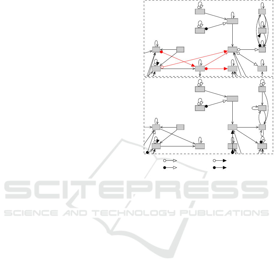
A cutout of the identiﬁed network is shown in Fig-

ure 2 for both concentrations. In general the apoptotic

pathways consists of the extrinsic pathway and the in-

trinsic one. Here the extrinsic one is shown in de-

tail. The expectation, that the concentration of T5µM

leads to apoptosis, while that of T50nM does not, is

afﬁrmed here. According to the database the extrinsic

pathway is triggered by engagements at the death lig-

ands, which activate caspase-8. That induces a signal-

ing cascade, resulting in an activation of caspase-3,

T5µM

Fadd

Tradd

Cﬂar

Capn1

Capn2

Casp8

Casp12

Casp3

Casp7

CAD

Dffb

Dffa

Casp6

T50nM

Fadd

Tradd

Cﬂar

Capn1

Capn2

Casp8

Casp12

Casp3

Casp7

CAD

Dffb

Dffa

Casp6

s = 0, v = 0 s = 0, v = 1

s = 1, v = 0 s = 1, v = 1

Figure 2: Identiﬁed extrinsic pathway for T5µM and

T50nM with given clustering constraints, (canalyzing func-

tions in red canalyzing functions, with no constraints in

black, that with minimum error is shown).

what leads to cell death. This can be seen for T5µM,

where caspase-8 is activated leading to and activation

of caspase-3. In Figure 2 the connections of impor-

tance here are marked in red. For T50nM there is

no connection between caspase-8 and caspase-3 de-

tected. The arcs with circled tail and triangular head,

denote the canalyzing genes, thus the major inﬂuenc-

ing one. If the tail is colored, its canalyzing value

is one, if the head is colored, the canalyzing value is

one, and zero otherwise. Thus, for the interconnec-

tion from caspase-8 to caspase-7 in the network of

T5µM this, e.g. means that an activation of caspase-

8 always activates caspase-7, irrespectively of other

genes, whereas a deactivation of Tradd always acti-

vates caspase-3.

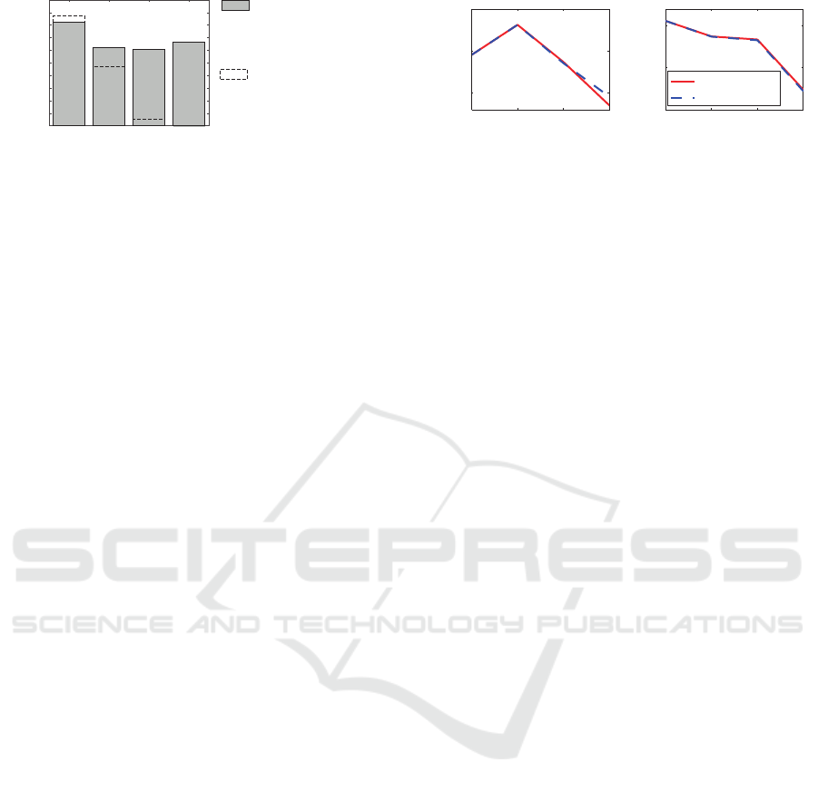
An a posteriori analysis of the models identiﬁed

by the identiﬁcation, where no canalyzing constraints

were imposed, shows that a signiﬁcant ratio of identi-

ﬁed models are canalyzing functions. These ratios of

canalyzing functions compared to all identiﬁed func-

tions for a certain connectivity degree are shown in

Figure 3. For comparison the overall ratios of canaly-

zing function in all Boolean functions, as calculated

from Table 1, are given. It is obvious that expect for

the connectivity degree of two the identiﬁed models

SIMULTECH 2016 - 6th International Conference on Simulation and Modeling Methodologies, Technologies and Applications

116

0.2

0.4

0.6

0.8

2 3 4 5

replacements

connectivity degree

ratio of canalyzing func-

tions resulting from the

identiﬁcation without ca-

nalyzing constraints

ratio of canalyzing func-

tion in all Boolean func-

tions

ratio of canalyzing

functions

Figure 3: Ratio of canalyzing functions.

show a signiﬁcant higher ratio of canalyzing functions

than there exists in total. This conﬁrms the choice to

restrict the identiﬁcation to canalyzing functions, not

only due to the restricted search space and thus re-

duced calculation time, but also because genetic mod-

els obviously tend to be canalyzing, as also reported

by biologists.

The identiﬁcation is repeated, without consider-

ing the dependency sets given by the database, but

testing all possible clusters with connectivity degree

from two to four with maximum number of rows of

the OTVL restricted to two. Note that thus for one

gene,













= 1505504 different clusters

have to be checked. Here only identiﬁcation with ca-

nalyzing constraints is performed, since without con-

straints, this is not tractable anymore. For T5µM in

average an error of 6.87×10

−5

is achieved, where

the root mean square error is taken as error measure.

Biologists talk about good approximations if an er-

ror < 10

−3

is achieved. This is not reached for only

two out of the 78 genes. Remark that for the identi-

ﬁcation the maximum number of lines of the identi-

ﬁed OTVLs was restricted to two, which is necessary

to reduce the solution space and make the problem

tractable. This seems to be very small. Nevertheless

the very good ﬁt of the identiﬁed models conﬁrms that

this might be enough. For T50mM the average error

is with 1.43×10

−4

slightly larger. This also let sus-

pect, that the high concentration rather lead to apop-

tosis than the low one. Here only the genes involved

in apoptosis are considered, but if other processes are

executed, other genes may be involved.

To analyze the continuous gene expression level

dynamics, the measurements and the prediction using

the identiﬁed model are compared. The prediction of

gene l, initialized with the measured values

y(0), is

determined by

(t + 1) = p

(y(t)) with y(0) =

y(0).

The dynamic of two genes for T5µM is shown in

Figure 4. Here with caspase-3 and caspase-8 , two

genes right in the center of the extrinsic pathway are

depicted. The prediction ﬁts very well, what is not

astonishing since errors of 1×10

−7

and 5.6×10

−8

0 . 7 5

0 . 8

0 . 8 5

0 1 2 3

discrete timesteps

gene expression data

caspase-3

0 1 2 3

0 . 5

0 . 5 5

0 . 6

discrete timesteps

gene expression data

caspase-8

measurement

prediction

Figure 4: Measured vs. predicted gene expression level dy-

namics for T5µM.

are achieved. For the sample T50nM the error of the

identiﬁed model is with 1. 2 ×10

−4

and 3.2×10

−4

al-

most 10

-times worse. This also supports the conclu-

sion, that other processes then apoptosis with other

genes involved occur for that sample.

6 CONCLUSIONS

The paper presents how to express canalyzing func-

tions in terms of OTVLs. Based on that, it is shown

how to restrict the solution space of the Boolean iden-

tiﬁcation algorithm in Lichtenberg and Eichler (2011)

to canalyzing functions by simple adaptions mainly

in the initialization step. Thereby the restriction to a

maximum number of lines, that as a core of the algo-

rithm leads efﬁciently to a suboptimal solution, does

not need to be given up. The advantage of the restric-

tion to canalyzing function is twofold, ﬁrst from the

biological point of view, since canalyzing functions

are known to describe gene networks better than other

functions, and second from the computational point of

view. By the adaption of the Zhegalkin identiﬁcation

algorithm presented in this paper, the search space

is enormously reduced by the canalyzing constraints,

what leads to managable computation times even for

larger data. The presented algorithm has been applied

to experimental gene data. By the canalyzing con-

straints the problem of identiﬁcation and clustering

of 78 genes got tractable and has shown very good

ﬁts. Further assumptions of the biologists regarding

the network structure of speciﬁc processes could be

approved by the algorithm presented here.

ACKNOWLEDGEMENTS

The authors acknowledge Saskia Trump (UFZ

Leipzig) for her support and experimental data.

Parameter Identiﬁcation of Canalyzing Boolean Functions with Ternary Vectors for Gene Networks

117

REFERENCES

Bochmann, D. and Steinbach, B. (1991). Logikentwurf mit

XBOOLE. Verlag Technik.

Breindl, C., Chaves, M., and Allg¨ower, F. (2013). A linear

reformulation of boolean optimization problems and

structure identiﬁcation of gene regulation networks. In

Proc. 52nd IEEE Conf. Decision Control, pages 733–

738.

Faisal, S. (2008). Discrete-Time Modelling of Gene

Networks by Zhegalkin Polynomials. Ingenieurwis-

senschaften. Dr. Hut Verlag.

Faisal, S., Lichtenberg, G., Trump, S., and Attinger, S.

(2010). Structural properties of continuous represen-

tations of boolean functions for gene network mod-

elling. Automatica, 46(12):2047–2052.

Faisal, S., Lichtenberg, G., and Werner, H. (2005). A poly-

nomial approach to structural gene dynamics mod-

elling. In Proc. 16th IFAC World Congr., pages 2119–

2119.

Faisal, S., Lichtenberg, G., and Werner, H. (2006). Canali-

zing Zhegalkin polynomials as models for gene ex-

pression time series data. In Proc. 1st Int. Cong. Eng.

Intell. Syst.

Jarrah, A. S., Raposa, B., and Laubenbacher, R. (2007).

Nested canalyzing, unate cascade, and polyno-

mial functions. PhysicaD: Nonlinear Phenomena,

233(2):167–174.

Kanehisa, M. and Goto, S. (2000). Kegg: Kyoto encyclo-

pedia of genes and genomes. Nucleic Acids Research,

28(1):27–30.

Kauffman, S. (1993). The Origins of Order, Self Organi-

zation and Selection in Evolution. Oxford University

Press.

Kauffman, S. A., Petersen, C., Samuelsson, B., and Troein,

C. (2003). Random boolean network models and the

yeast transcriptional network. PNAS, 100(25):14796–

14799.

Kolda, T. and Bader, B. (2009). Tensor decompositions and

applications. SIAM Review, 51(3):455–500.

Lichtenberg, G. and Eichler, A. (2011). Multilinear alge-

braic boolean modelling with tensor decompositions

techniques. In Proc. 18th IFAC World Congr., pages

5603–5608.

Lichtenberg, G., Faisal, S., and Werner, H. (2005). Ein

Ansatz zur dynamischen Modellierung der Genex-

pression mit Shegalkin-Polynomen. Automatisierung-

stechnik, 53:589–596.

Lin, P. and Khatri, S. (2013). Logic Synthesis for Genetic

Diseases: Modeling Disease Behavior Using Boolean

Networks. Springer.

Veliz-Cuba, A., Jarrah, A. S., and Laubenbacher., R. (2010).

Polynomial algebra of discrete models in systems bi-

ology. Bioinformatics, 26(13):1637–1643.

Zhegalkin, I. (1928). Arithmetics of symbolic logic. Mat.

Sb., 35(3-4):311–377.

SIMULTECH 2016 - 6th International Conference on Simulation and Modeling Methodologies, Technologies and Applications

118