
Learning Global Inverse Statics Solution for a Redundant Soft Robot
Thomas George Thuruthel
1
, Egidio Falotico
1
, Matteo Cianchetti
1
, Federico Renda
2
and Cecilia Laschi
1
1
The Biorobotics Institute, Scuola Superiore Sant’Anna, Pisa, Italy
2
KURI Institute, Khalifa University, Abu Dhabi, U.A.E.
Keywords: Soft Robots, Machine Learning, Inverse Statics, Inverse Dynamics, Steady State Model, Neural Networks.
Abstract: This paper presents a learning model for obtaining global inverse statics solutions for redundant soft robots.
Our motivation begins with the opinion that the inverse statics problem is analogous to the inverse
kinematics problem in the case of soft continuum manipulators. A unique inverse statics formulation and
data sampling method enables the learning system to circumvent the main roadblocks of the inverting
problem. Distinct from previous researches, we have addressed static control of both position and
orientation of soft robots. Preliminary tests were conducted on the simulated model of a soft manipulator.
The results indicate that learning based approaches could be an effective method for modelling and control
of complex soft robots, especially for high dimensional redundant robots.
1 INTRODUCTION
Continuum soft robots are a class of robots made of
soft materials that exhibit highly dexterous and
adaptive behaviour. Not a lot is known about the
dynamic behaviour of continuum robots. They are
inherently difficult to control, due to their
compliance. However, they have some
characteristics which make certain tasks easier for
them. Their compliant nature makes them
frontrunners for applications involving interactions
with delicate or unstructured environment (Rus et al.,
2015).
As a growing field in robotics, there are
numerous challenges restricting the application of
soft robots. One of them is the construction of
inverse models for their kinematic and dynamic
behaviour. IK models have the advantage that their
solutions are load independent. However, our
interest lies on modelling the inverse steady state
dynamics (statics) of these robots, specifically for
redundant soft manipulators. We believe that hybrid
controllers with coupled inverse kinematic solvers
and inverse statics (IS) solvers would be exciting for
soft robotics applications. They can be used in
tandem for position control and force/stiffness
estimation.
Theoretically, due to their continuous nature, soft
robots have an infinite number of degrees of
freedom, making them under-actuated. Assuming
that there are no external forces, we can still develop
a mapping between the applied internal forces and
the configuration of the robot very much like the
case of kinematics. However, developing an inverse
model poses more difficulties. Similar to the inverse
kinematic formulation of rigid redundant robots, the
inverse statics solution is not unique and the solution
set forms a non-convex set (D’Souza at al., 2001).
Furthermore, analytical or numerical methods
appear to be very complex unless developed with
simplified models (Marchese e al., 2014). We are,
therefore, adopting a method based on machine
learning for estimating these models.
Inverse statics models are meaningful only for
soft manipulators and parallel robots because of the
existence of a stable zero velocity fixed point.
Essentially, the IS model is analogous to the IK
model for rigid robots. Therefore, numerous
approaches developed for IK problem of redundant
rigid robots can be directly used for our case.
Among the learning based approaches, a common
theme is the use of locally linear models and
stitching them together to form a global estimate.
This can be done in the velocity level and has been
widely used (D’Souza et al., 2001; Susumu et al.,
2001; DeMers et al., 1992). However, differential IK
methods involve integration over time to obtain
position estimates which can lead to accumulation of
Thuruthel, T., Falotico, E., Cianchetti, M., Renda, F. and Laschi, C.
Learning Global Inverse Statics Solution for a Redundant Soft Robot.
DOI: 10.5220/0005979403030310
In Proceedings of the 13th International Conference on Informatics in Control, Automation and Robotics (ICINCO 2016) - Volume 2, pages 303-310
ISBN: 978-989-758-198-4
Copyright
c
2016 by SCITEPRESS – Science and Technology Publications, Lda. All rights reserved
303

errors. Alternatively, a position level IK solution
was proposed using goal babbling (Rolf et al.,
2013a). However, this method generates only a
particular global solution and requires lot of sample
data. Inverting a learned forward model was carried
out by distal supervised learning by few researchers
(Jordan et al., 1992; Melingui et al., 2014). However,
these methods have not scaled well for higher
dimensional systems. Position level IK solution has
been proposed using modular learning architectures
by few other researchers (Vannucci et al., 2014;
2015), but it involves very complex constructions.
In this paper we propose an approach for
learning the global inverse statics model for a
continuum robot. Our method is also based on the
locally linear and convex properties of the IS
solution. However, we further utilize the fact that
these local models can be scaled and used as a
decent approximation of the global solution. This
can be achieved by appropriate biasing and selection
of the input/output representation of the learning
system. We are using neural networks to
approximate the proposed IS mapping. Giorelli et al.,
(2015), were one of the first researchers to propose
the learning of the inverse statics of soft arm. They
were successfully able to learn the inverse statics for
the position control of a soft robot. However, their
study was limited to the case of a non-redundant
manipulator and further restricted to only position
control (three Degrees of Freedom). Therefore, this
paper proposes a method for obtaining the global
solutions for both position and orientation of a soft
redundant robot. We have tested and validated the
proposed method on a simulated steady state model
of a 12 Degrees of Freedom (DoF) soft manipulator.
We have tried to show by simulations that the
proposed method performs soundly even with the
issues of redundancy and high dimensionality.
Further, we try to investigate the underlying form of
the learned system and compare it with the
commonly used inverse Jacobian based method.
2 PROPOSED METHOD
The forward static model or steady state model can
be represented by:
(1)
Where, ∈
is the position and orientation
vector; ∈
is the vector containing the actuator
tensions; and is some surjective function. This
particular representation is not invertible whenm
n (redundant). As mentioned before, we can develop
local representations by linearizing the function at a
point (
), thereby obtaining;
(2)
Here,
is the Jacobian matrix at the point
;
and are infinitesimally small changes in and
respectively. The differential IK method involves
generating samples of (,,) and learning the
mapping (,
) →.Thelearningisfeasible
sincethedifferentialIKsolutionsformaconvex
setandthereforeaveragingmultiplesolutions
stillresultsinavalidsolutionD’Souzaetal.,
2001.Themethodwehaveproposedinvolves
expandingEq.2andexpressingitintermsof
absolutepositions,asshownbelow:
(3)
Here,
is the next actuator configuration for
reaching a point
from the present
configuration
. Note that Eq. 3 is only valid when
the configurations are infinitesimally close.
However, for practical purposes this can be a good
approximation for larger regions. The analytical
solution for Eq. 3 can be written as:
(4)
Where,, is a generalized inverse of
and
is
the identity matrix and is an arbitrary n-
dimensional vector. The first component represents
the particular solution to the non-homogenous
problem prescribed in Eq. 3 and the second
component represents the infinite homogenous
solutions. It can be proved that the solution space
still forms a convex set. Therefore, any universal
function approximator can be used for learning the
mapping (
,
)→
. Setting the vector to
zero and using the Moore-Penrose pseudoinverse
provides us with the minimum norm ( ∥
∥)
solution to the linear eq. 3.
The samples (
,
,
) generated are such
that∣
∣ϵ. An appropriate value of ϵis
between 10%5% of the maximum actuator range.
The advantage of this reformulation is in the simple
detail that the input/ output domain of the learning
system is now same as the actuator space and task
space configuration and not a subset of it, unlike the
differential IK method. We predict that this way our
proposed method will behave exactly like the
differential IK method at local regions and at farther
points they will automatically provide approximate
configurations that will bring the end effector
configuration closer to the target. Therefore if we
repeat the process for a fixed target, we can expect
the process to converge near the target position.
ICINCO 2016 - 13th International Conference on Informatics in Control, Automation and Robotics
304
Therefore, by our method we can get global
solutions for the IS problem. We can further add
constraints during the iteration process to develop
particular solutions for the IS problem according to
our requirement.
2.1 Reachability and Workspace
Considerations
Since, the IS solution will provide the actuator
configuration to take the end effector to a particular
position and orientation, it is important to know if
the input arguments (
) given to the system is
reachable. For the case of end effector position, the
reachable workspace will describe the volume in
which the end effector position can reach. The
reachable workspace can be estimated easily either
by analytical, numerical or experimental methods.
However, the dexterous workspace, which describes
the volume in which the end effector can reach with
all orientations, is much more difficult to find.
Nonetheless, the calculation of the dextrous
workspace is not of significance for soft robots.
Dextrous workspace is a property introduced
primarily for rigid robots with spherical joints. For
soft robots, the manifold of reachable orientation
varies according to the end effector position.
Interestingly, there exists a single unique
manifold for each position, unlike the case of rigid
robots which can have multiple disjoint manifolds
(Kapadia et al., 2013). This is attributed to the fact
that for soft continuum robots, singular
configurations arise only when the manipulator has
zero curvature. Singularities at boundaries can be
ignored since the manipulator can, theoretically,
extend or contract to any length. Furthermore, in our
formulations, we are neglecting rotations along the
backbone of the robot (roll). So, our robot can be
visualized as a ‘pointing’ robots (rotations in
3
are replaced by directions in
). By this
process our formulation is theoretically devoid of
singularities. This implies that given a current
positon and orientation (
,
), there exists a
continuous path in the actuator space, which can
bring the end effector to a different orientation
(
,
), without affecting the position. Learning the
null space solution for each end effector
configuration will help us in implementing this.
However, learning the null space from just
experimental data is very difficult. Therefore, in this
paper we have developed two solvers for the IS
problem; one for both position and orientation and
the other for just the orientation. These two solvers
can be combined appropriately to attain the required
accuracies in position and orientation. For instance,
if the network output for coupled (position +
orientation) IS solver is
and the output for
Inverse Orientation Statics (IOS) solver is
,
then, they can be combined to give actuator
configuration
, where;
∗
1
∗
(5)
By regulating the value of the constant1,
we can accordingly vary the orientation accuracy. In
further sections we will be referring to this
formulation as the appended IS solver and the
complete IS solver will be just referred to as the IS
solver.
3 STEADY STATE MODEL
The constant curvature model is the most widely
used construction technique for soft robots due to
their simplicity and computational ease (Walker,
2013). Non- constant curvature models based on
cosserat beam dynamics promises to be a better
alternative (Renda et al., 2014). For our application,
we have used a steady state model of a tendon
driven soft continuum robot (Renda et al., 2012).
The sample data for learning the IS model is
obtained from this steady state model.
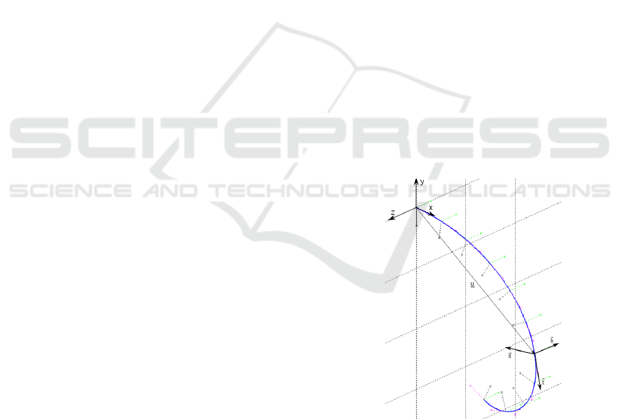
Figure 1: Kinematic representation of the cosserat beam
model.
The soft continuum robot is modelled as a
cosserat beam. A cosserat beam can be visualized as
a continuum body which is composed of
infinitesimally small rigid bodies that can rotate
independently from the neighbouring element. The
position and orientation of each material element is
Learning Global Inverse Statics Solution for a Redundant Soft Robot
305
represented by four vectors: ,,,. The unit
vector is tangential to the manipulator backbone at
that section and the vectors and lie on the cross
sectional area of the element. These three unit
vectors form the local reference frame for each
element. Therefore, the relation holds
true everywhere. is the position vector of the
centre of mass of an element (Fig. 1). We are
ignoring the effects of shear stresses in our
formulation (Euler-Bernoulli hypothesis). This
restricts the DoF of each element to four. The total
length of our manipulator is 31 centimetres, divided
into a section per centimetre.
The complete configuration of the robot can be
calculated by obtaining the four vectors for each
element. The elements are related to each other in
space by the below equations (Renda et al., 2012):
1
1
(6)
1
1
(7)
1
1
(8)
1
(9)
Here the functions
and
are the curvatures
with respect to
and
,
is the torsion
with respect to
, and
is the longitudinal
strain along the arm.
, is the parametrization
variable which represents an element.
The variables
,
,
and
are
related by the following equations:
0 0
0
0
00
00
0
0
00
(10)
(11)
EA
(s)
Where, (s) is the component of the internal
contact forces and is the vector of the internal
torque forces (The dot symbol is the derivative with
respect to s). is the Young’s modulus, is the
shear modulus, ,
and
are the moment of inertia
of the section with respect to,and, in that order.
The internal contact forces and the internal torque
forces are calculated based on the cable
configuration and tension on each cable (Refer to
Renda et al., 2012). Equation 10 is numerically
integrated from tip to base and solved along with
equation 11 and appropriate boundary conditions to
obtain the curvatures and strains in each segment.
Finally, the kinematic equations 6, 7, 8, 9 are
integrated to obtain the arm shape.
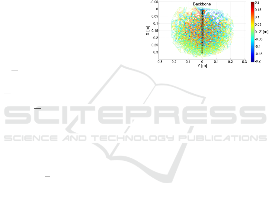
There are three anchorage planes along the
length of the manipulator. Each anchorage plane has
four cables attached to it; each spaced apart by an
angle of 90 degrees. Fig. 2 shows the reachable
workspace of the robot obtained by random
exploration in the actuator space.
Figure 2: Schematic of the robot end effector workspace.
4 DATA COLLECTION AND
TRAINING
The samples (
,
,
) are generated by motor
babbling. The distance between consecutive samples
(
) is decided randomly from a range to
avoid any bias in the sample. The range of the each
sampling data is from zero to 8 percent of the
maximum actuator force. The range is decided by
trial and error. Learning with a lower range will give
better accuracy, but requires larger data set and
performs poorly for farther target points. Therefore a
continuous path must be planned beforehand, just
like the case of differential IK. Selecting the distance
from a range rather than a fixed value keeps the
continuous nature of the problem intact, at least
partially. Note that there are 12 actuators which can
select its actions continuously. Even if we consider
that the actuator space is discretized into 12
segments (each segment being roughly 8 percentage
of the total range), there are still around 9e+12
possible configurations. Therefore, we cannot
navigate the whole actuator space, instead we expect
the generalization ability of neural networks or other
machine learning process’s to predict accurate
solutions for unseen data.
4.1 Training
As mentioned before, we are using neural networks
ICINCO 2016 - 13th International Conference on Informatics in Control, Automation and Robotics
306
to learn the mapping (
,
) →
. The input
layer is of size 18 for the IS solver and 15 for the
IOS solver. The output layer size is 12 for both cases.
We are using a multilayer perceptron with a single
hidden layer for this. Tan-sigmoid activation
function is used in the hidden layer and a linear
activation function is used at the output layer. Proper
care must be taken during the training process.
Bayesian regularization backpropagation method is
used for training the neural network (Foresee at al.,
1997). The inputs and outputs are normalized and
divided randomly in the pre-processing stage. A
uniformly distributed noise is also added to the
inputs to imitate realistic scenarios. The magnitude
of the noise goes up to 3% of the maximum
sampling range. Since the Bayesian regularization
backpropagation algorithm is used for training; the
data set is divided into training and test set in the
ratio 80:20. No validation set is used. In the
following subsections we describe the methodology
adopted for determining the network size and sample
data size for learning the IS. The parameters of the
IOS solver are adopted from the IS solver as it can
be seen as a subset of the IS problem.
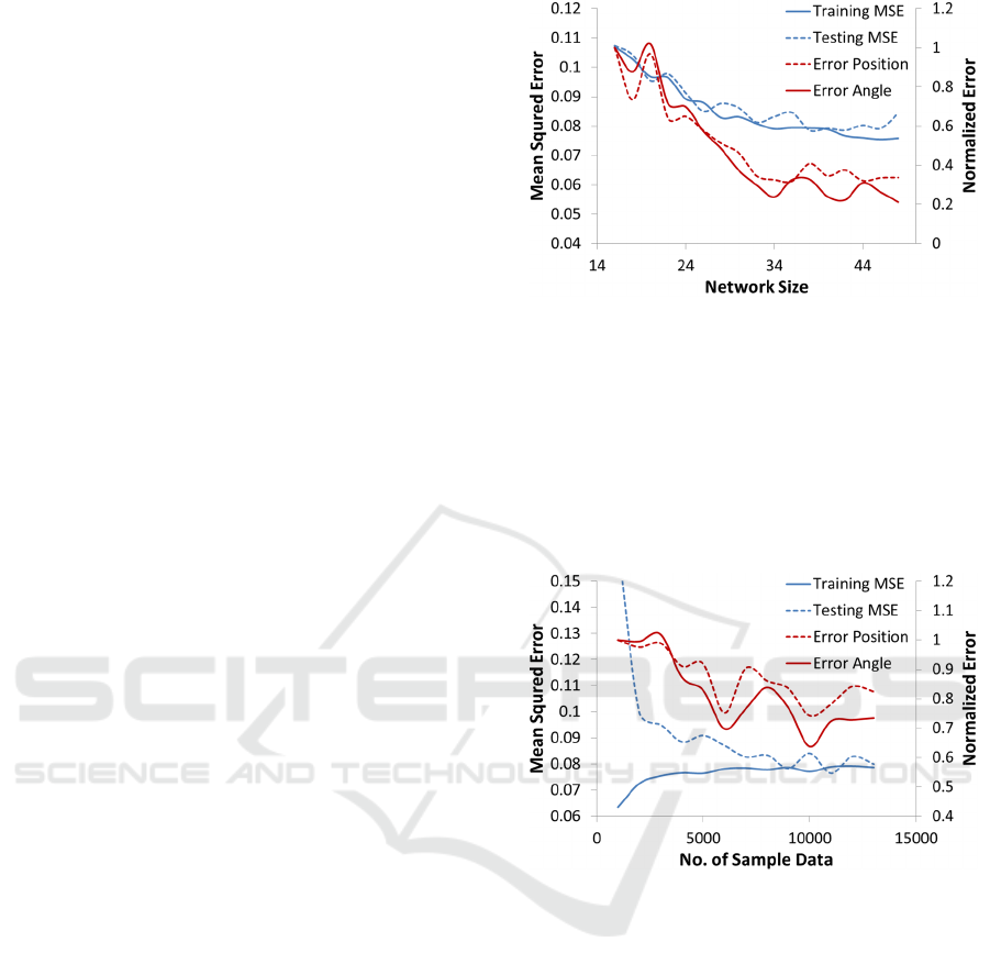
4.1.1 Network Size
Proper care must be given to decide the hidden layer
size. It is not enough to get good training or test
performance, contrary to common intuition. The
learning task provided to the neural networks is to
learn a left inverse function. However, our objective
is to learn the right inverse function (Rolf et al.,
2013b). In other words, the neural network tries to
reduce the error between the predicted values
of
and the sample values of
.
Whereas, the final aim is to reduce the error between
and
. There are local minima which can
provide good training and test performance, and still
perform poorly as a IS solver. For instance, a
network that outputs
, can give good
training and test performance as both values are
nearby due to the sampling method. Therefore, the
appropriate size for the network is decided by
checking the training error along with the
performance of the IS solver. Fig.3 shows effect of
network size on the training performance and the
corresponding change in the IS performance. IS
solver performance is measured by testing the
solutions for fifty points randomly selected from the
sample data (to ensure that the targets are reachable).
Figure 3: Network size determination. The errors in
position and angle are normalized for easier comparison.
4.1.2 Sample Size
The length of the sample data required would be
directly proportional to the number of DoF’s of the
system. Fig. 4 shows how the number of samples
determine the performances of the network and the
IS solver.
Figure 4: Sample data size determination. The network
size is forty for all tests.
For all the ensuing experiments we have selected
14000 samples for training a neural network of size
40 units. Note that the proposed method needs to
explore only a miniscule percentage of the actuator
space. The same analysis cannot be done
independently for IOS solver since the performance
of the IOS solver is heavily dependent on the
position of the manipulator (Reachability of a
particular orientation depends on the corresponding
position). Therefore, the performance of the IOS
solver can only be inspected with the help of the IS
solver. However, since we are using Bayesian
regularization backpropagation algorithm for
training the network, an exaggerated network size
and sample data will not harm the learning process.
Therefore, the same parameters of the IS solver was
adopted for the IOS solver.
Learning Global Inverse Statics Solution for a Redundant Soft Robot
307
5 RESULTS AND ANALYSIS
This section is divided into three subsections; the
first subsection shows the test results for the
developed IS solver on the simulated steady state
model; the second subsection discusses the results
with the appended IS solver (Sec. 2.1); the final
subsection makes a comparative analysis of the
proposed method with the inverse Jacobian method.
There are two reasons for this; the first one is to
compare the performance of the two methods;
secondly, the comparison can help us understand the
underlying form of the learned network.
5.1 Simulations
The main advantage of the proposed method is its
ability to provide global solutions to the IS problem
without the need to pre-plan a path from the starting
point. So, the first tests were to evaluate if the IS
solver can provide accurate actuator configuration
for random target points in the workspace. Fifty
points ( x∈
0.05,0.35
,y∈
0.25,0.25
,z∈
0.2,0.2)) were randomly selected from the sample
data along with their corresponding orientation.
Since the target points are not close to the home
position (0.31[m], 0[m], 0[m]), the solver needs
more than one iteration for converging to the right
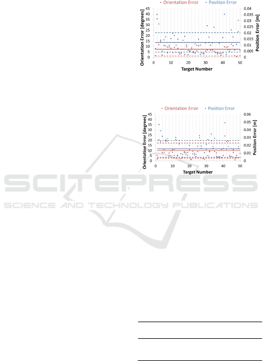
solution. Fig. 5 shows the test results for this
experiment. The proposed method is able to generate
results with a mean positional error of 0.012 meters
and mean orientation error of 7.4 degrees. The
method converges with an average of 3.56 steps for
convergence within a range of 1mm. The same fifty
target points were again used in the IS solver for a
starting point at one of the extreme boundary points
(-0.02[m],-0.16[m],-0.01[m]). The corresponding
results are shown in Fig. 6. The average errors
increase in this case. The average positional error
goes to 0.015 meters and the average orientation
error goes to 9.92 degrees. The convergence speed
remains the same with each target taking an average
of 3.68 iterations for convergence. Note that even
though the magnitude of error increases, the error
pattern remains relatively similar. We suggest that
these points are under-represented in the sample data
and therefore the learning system does not have an
adequate representation around that region. One
possible work-around is to develop algorithms that
perform motor babbling initially and then later
switch to a more goal oriented exploration strategy.
Figure 5: Simulation results for the fifty points experiment
at the natural starting point. The thick lines represent the
mean of the data and the dotted lines on either side of the
mean represent the standard deviation.
Figure 6: Simulation results for the fifty points experiment
for a starting point at one of the boundary extrema.
The next set of simulations were conducted for
continuous targets, i.e. the target points are locally
adjacent and therefore forms a continuous path. As
the target points are close by, the IS solver can
output a solution in one iteration. Two such paths
were used for evaluation. The first one is a circular
path of radius 0.1 meters, centered at (0.25[m], 0[m],
0[m]), with a fixed orientation parallel to the X axis
(Fig. 7). The other path is a fixed point with a
continuous change in elevation (0→90→0 degrees)
and azimuth (0→180 degrees). Fig. 8 shows the
target orientation vectors for this simulation and the
corresponding solutions from the IS solver. For both
tests, the manipulator starts from the home position
(Zero force position). The results of both tests are
encapsulated in Table 1.
Table 1: Continuous path results.
Test
Position Error
(Mean
Standard
Deviation) [m]
Orientation Error (Mean
Standard Deviation)
[degrees]
Circular
Path
0.0085 0.0028 7.33 3.98
Angular
Path
0.0118 0.0059 3.21 1.71
ICINCO 2016 - 13th International Conference on Informatics in Control, Automation and Robotics
308
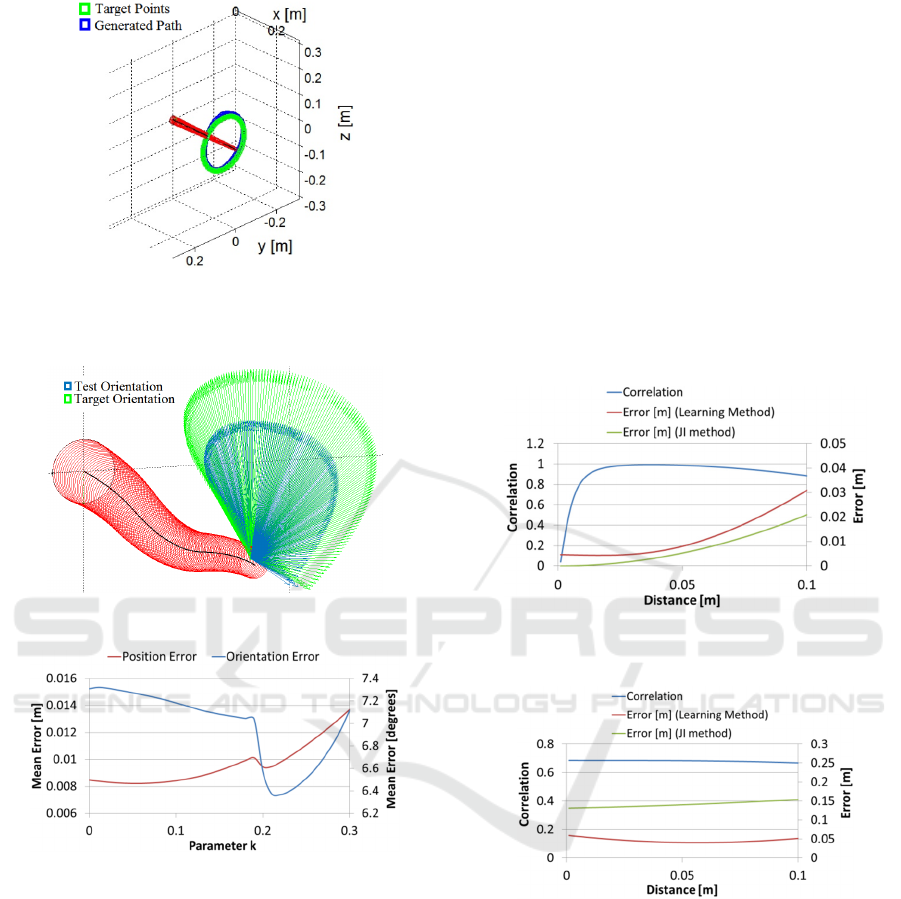
Figure 7: Continuous positional path following with fixed
orientation. The target orientation is a vector perpendicular
to the YZ plane.
Figure 8: Continuous angular path following.
Figure 9: Appended IS solver.
5.2 Appended IS Solver
As mentioned in the subsection 2.1, redundant soft
manipulators have certain geometrical properties
that could allow smooth motions in the self-motion
manifold. The continuous positional path experiment
(Fig.7) was again used to test the appended IS solver.
Fig. 9 depicts how the modified solver can allow us
to trade-off between positional accuracy and
orientation accuracy, leading to an improvement in
orientation accuracy by 0.95 degrees and reduction
of positional accuracy by 1.3 mm.
5.3 Analysis
The proposed methodology for learning the IS of a
redundant soft manipulator is an adaptation of the
differential IK/IS method. Therefore, we try to make
a comparison to the differential IK/IS method. The
Jacobian at a point (Equation 2) can be obtained
numerically by making infinitesimally small changes
in the actuator configuration and observing the
corresponding changes in the end effector
configuration. Once the Jacobian matrix is obtained,
it is inverted to obtain a particular solution to the
IK/IS problem. For a redundant manipulator, the
Moore-Penrose pseudo inverse will achieve the
same. We ignore the null space solutions in this
analysis.
Figure 10: Correlation between the proposed method and
JI method for a starting point at the home position.
Figure 11: Correlation between the proposed method and
Jacobian inverse method starting at a boundary extremum.
We compare the correlation between the
solutions provided by a Jacobian pseudo inverse (JI)
based method and our proposed method at two
points. One is the natural home position and the
other is a boundary extremum. The correlation
between the Inverse Jacobian method and the
proposed method for varying target distance is
shown in Fig. 10. We can observe that the
correlation between the Jacobian pseudo inverse
method and the learned system is high at the home
position. This implies that the system tends to learn
the ‘shortest path’ solution. It is low at lower
Learning Global Inverse Statics Solution for a Redundant Soft Robot
309

distances possibly because of the added noise. The
trend is similar for other points well within the
boundary. However for a starting position that lies at
one of the extremum of the workspace, the
correlation value is less (Fig. 11). The proposed
method also performs better than the Inverse
Jacobian method.
6 CONCLUSIONS
This paper presents a data driven method for
learning the inverse statics mapping of a redundant
soft manipulator. The novelty in our methodology
arises from our linearized IS problem reformulation
and sampling approach while implicitly feeding the
learning system with information about the system
boundaries. We have demonstrated through
simulations that the proposed approach is suitable
for static control of high dimensional redundant soft
manipulators. We have also tried to address the
possibility of utilizing the distinct self-motion
manifolds of soft robots and its probable
implications. Finally, comparison of the proposed
method with commonly used inverse Jacobian
method indicates that the learning system
generalizes to the ‘shortest path’ solution.
ACKNOWLEDGEMENTS
The authors would like to acknowledge the support
by the European Commission through the I-
SUPPORT project (HORIZON 2020 PHC-19,
#643666).The authors would like to thank Italian
Ministry of Foreign Affairs and International
Cooperation DGSP-UST for the support through
Joint Laboratory on Biorobotics Engineering project.
REFERENCES
Demers, D., Kreutz-Delgado, K., 1992. Learning Global
Direct Inverse Kinematics. Advances in Neural
Information Processing Systems, 589-595.
D’Souza, A., Vijayakumar, S., Schaal, S., 2001. Learning
Inverse Kinematics. In Proc IEEE/RSJ International
Conference on Intelligent Robots and Systems,
Volume 1, 298 – 303.
Foresee, F. D., Hagan, M. T., 1997. Gauss-Newton
approximation to Bayesian regularization. In Proc.
1997 International Joint Conference on Neural
Networks, 1930–1935.
Giorelli, M. et al., 2015. Neural Network and Jacobian
Method for Solving the Inverse Statics of a Cable-
Driven Soft Arm with Nonconstant Curvature. IEEE
Transactions on Robotics, 31(4), 823 – 834.
Jordan, M., Rumelhart, D., 1992. Forward models:
supervised learning with distal teacher. Cognitive
Science, 16(3), 307–354.
Kapadia, A. D., Walker, I. D., 2013. Self-Motion Analysis
of Extensible Continuum Manipulators. IEEE
International Conference on Robotics and Automation,
1988 – 1994.
Marchese, A. D. et al., 2014. Design and control of a soft
and continuously deformable 2D robotic manipulation
system. In Proc. IEEE International Conference on
Robotics and Automation, 2189–2196.
Melingui, A. at al., 2014. Neural Networks based
approach for inverse kinematic modeling of a
Compact Bionic Handling Assistant trunk. IEEE 23rd
Int. Symposium on Industrial Electronic, 1239-1244.
Renda, F. et al., 2012. A 3D steady-state model of a
tendon-driven continuum soft manipulator inspired by
the octopus arm. Bioinspiration & Biomimetics, 7(2).
Renda, F. et al., 2014. Dynamic Model of a Multibending
Soft Robot Arm Driven by Cables, IEEE Transactions
on Robotics, 30(5): 1109 – 1122.
Rolf, M., Steil J.J., 2013a. Efficient Exploratory Learning
of Inverse Kinematics on a Bionic Elephant Trunk,
IEEE Transactions on Neural Networks and Learning
Systems, 25(6), 1147 – 1160.
Rolf, M., Steil, J.J., 2013b. Explorative learning of right
inverse functions: theoretical implications of
redundancy. Neurocomputing.
Rus, D., Tolley, M. T., 2015. Design, Fabrication and
control of soft robots, Nature 521: 467–475.
Susumu, E.O., Tachi, S., 2001. Inverse kinematics
learning by modular architecture neural networks. In
Proc. IEEE International Conference on Robotics and
Automation, 1006–1012.
Vannucci, L., Cauli, N., Falotico, E., Bernardino, A.,
Laschi, C., 2014. Adaptive visual pursuit involving
eye-head coordination and prediction of the target
motion. 14th IEEE-RAS International Conference on
Humanoid Robot, 541–546.
Vannucci, L., Falotico, E., Di Lecce, N., Dario, P., Laschi,
C., 2015. Integrating feedback and predictive control
in a Bio-inspired model of visual pursuit implemented
on a humanoid robot.
Lecture Notes in Computer
Science (including subseries Lecture Notes in
Artificial Intelligence and Lecture Notes in
Bioinformatics), 9222, 256-267.
Walker, I. D., 2013. Continuous Backbone ‘‘Continuum’’
Robot Manipulators, ISRN Robotics, vol. 2013.
ICINCO 2016 - 13th International Conference on Informatics in Control, Automation and Robotics
310
