Tracking of High-speed, Non-smooth and Microscale-amplitude
Wave Trajectories
Jiradech Kongthon
Department of Mechatronics Engineering, Assumption University, Suvarnabhumi Campus, Samuthprakarn, Thailand
Keywords: High-speed Tracking, Inversion-based Control, Microscale Positioning, Reduced-order Inverse, Tracking.
Abstract: In this article, an inversion-based control approach is proposed and presented for tracking desired
trajectories with high-speed (100Hz), non-smooth (triangle and sawtooth waves), and microscale-amplitude
(10 micron) wave forms. The interesting challenge is that the tracking involves the trajectories that possess a
high frequency, a microscale amplitude, sharp turnarounds at the corners. Two different types of wave
trajectories, which are triangle and sawtooth waves, are investigated. The model, or the transfer function of
a piezoactuator is obtained experimentally from the frequency response by using a dynamic signal analyzer.
Under the inversion-based control scheme and the model obtained, the tracking is simulated in MATLAB.
The main contributions of this work are to show that (1) the model and the controller achieve a good
tracking performance measured by the root mean square error (RMSE) and the maximum error (E
max
), (2)
the maximum error occurs at the sharp corner of the trajectories, (3) tracking the sawtooth wave yields
larger RMSE and E
max
values,compared to tracking the triangle wave, and (4) in terms of robustness to
modeling error or unmodeled dynamics, E
max
is still less than 10% of the peak to peak amplitude of 20
micron if the increases in the natural frequency and the damping ratio are less than 5% for the triangle
trajectory and E
max
is still less than 10% of the peak to peak amplitude of 20 micron if the increases in the
natural frequency and the damping ratio are less than 3.2 % for the sawtooth trajectory.
1 INTRODUCTION
A piezo stage is widely used in positioning and
actuating motions in nano/microscale displacements
or amplitudes. Several works have used a
piezoactuator to achieve the goals. For example, the
works done by Kongthon et al., (2010, 2011 and
2013) employed a piezo-based positioning system to
drive the biomimetic cilia-based device so that the
mixing performance in a micro device was
improved. Moallem et al., (2004) used piezoelectric
devices for the flexure control of a positioning
system.
The tracking of a trajectory is very common in
control problems such as the works by Beschi et al.,
(2014) and Martin et al., (1996). Tracking can be
challenging in high-frequency applications with very
small displacements. The challenge in this work is
that the trajectories are of high-speed (100Hz), non-
smooth (triangle and sawtooth waves), and
microscale-amplitude (10 micron) wave forms. The
goal is to propose a controller that can track
prescribed trajectories properly with a good tracking
performance. The tracking performance can be
measured by the root mean square error (RMSE) and
the maximum error (E
max
).
The rest of this article is structured as follows.
Section 2 introduces the two trajectories. The
piezoactuator model is obtained in section 3. The
control scheme is proposed in section 4. Section 5
shows the results. In section 6, the robustness is
investigated. Section 7 concludes the article.
2 TRAJECTORIES
2.1 The Trajectories to Be Tracked
In this work, there are two types of wave form
trajectories used to investigate the tracking
performance of the piezoactuator model: triangle
wave, shown in Fig. 1 and sawtooth wave, shown in
Fig. 2.
Kongthon, J.
Tracking of High-speed, Non-smooth and Microscale-amplitude Wave Trajectories.
DOI: 10.5220/0005979704990507
In Proceedings of the 13th International Conference on Informatics in Control, Automation and Robotics (ICINCO 2016) - Volume 1, pages 499-507
ISBN: 978-989-758-198-4
Copyright
c
 2016 by SCITEPRESS – Science and Technology Publications, Lda. All rights reserved
499

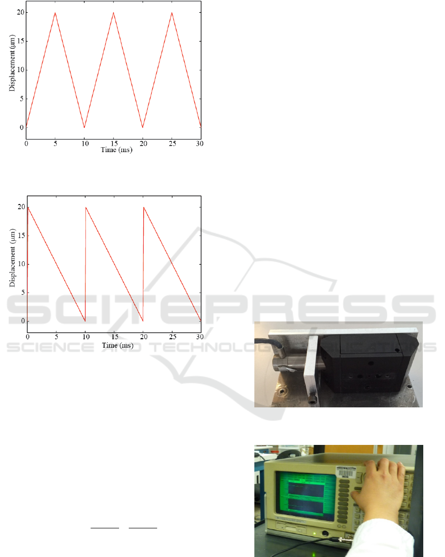
Figure 1: Original trajectory for triangle wave of 10
m
μ
amplitude and 100 Hz frequency
Figure 2: Original trajectory for sawtooth wave of 10
m
μ
amplitude and 100 Hz frequency
2.2 Filtered and Desired Trajectories
It can be seen in Figs. 1 and 2 that the original
trajectories contain very sharp turnarounds at the
corners. In practice, an actuator cannot track a
trajectory with a very sharp corner properly as it has
a limited bandwidth. In order to achieve a good
tracking performance, the original trajectories
therefore need to be smoothen by a second-order
filter with the filtering transfer function of the form.
⎟
⎟
⎠
⎞
⎜
⎜
⎝
⎛
+
⎟
⎟
⎠
⎞
⎜
⎜
⎝
⎛
+
=
f
f
f
f
f
ss
sG
ω
ω
ω
ω
)(
where
f
ω
is the break frequency of the filter , and In
this work,
f
ω
of 10 Hz, or
)2(10
π
rad/s is selected to
get the trajectories filtered. The filtered trajectory is
hereafter referred to as the desired trajectory. The
controller then needs to track the desired trajectory
of each type.
3 PIEZO ACTUATOR MODEL
A piezo-based positioning system, or piezo stage,
can be used in applications that require very small
displacements and large frequency ranges. A
piezoactuator can generate an extremely small
displacement down to the subnanometer range.
The number of vibration modes for the piezo
stage is infinite since the beam mechanism inside the
piezo stage has an infinite dimension. In general, an
infinite dimensional plant can be approximated by a
finite dimensional model, and in practice, it is
possible to take the first few modes of vibration to
represent the total dynamics of the plant.
3.1 Frequency Response Experiment
To obtain the model of the piezoactuator shown in
Fig. 3, the piezoactuator and the dynamic signal
analyzer shown in Fig. 4, together with an inductive
sensor and a power amplifier are connected as
shown in Fig. 5 to get the frequency response, and
the model is then obtained.
Figure 3: Piezoactuator used to produce micro-scale
amplitudes of oscillations with high frequencies.
Figure 4: Dynamic signal analyzer used to get the
frequency response to obtain the model of the actuator.
ICINCO 2016 - 13th International Conference on Informatics in Control, Automation and Robotics
500

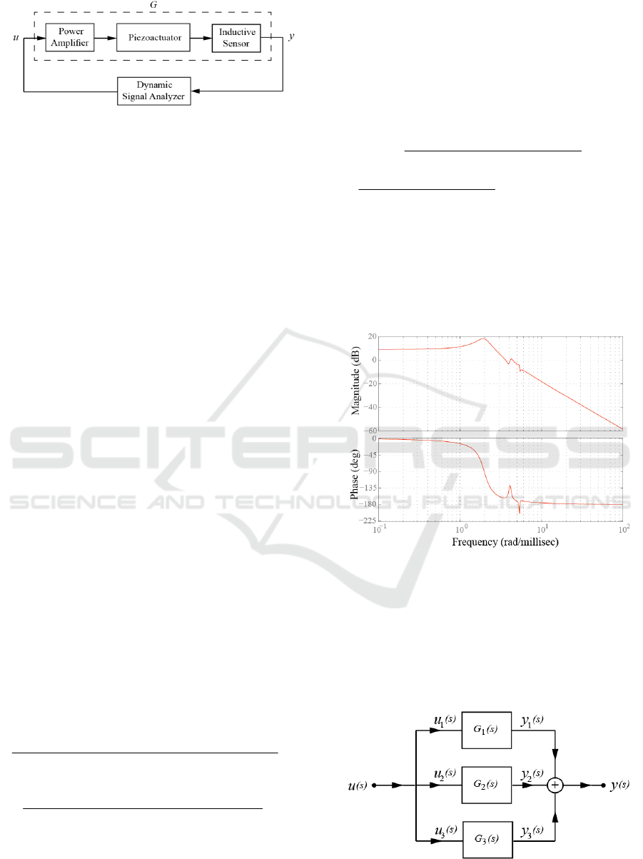
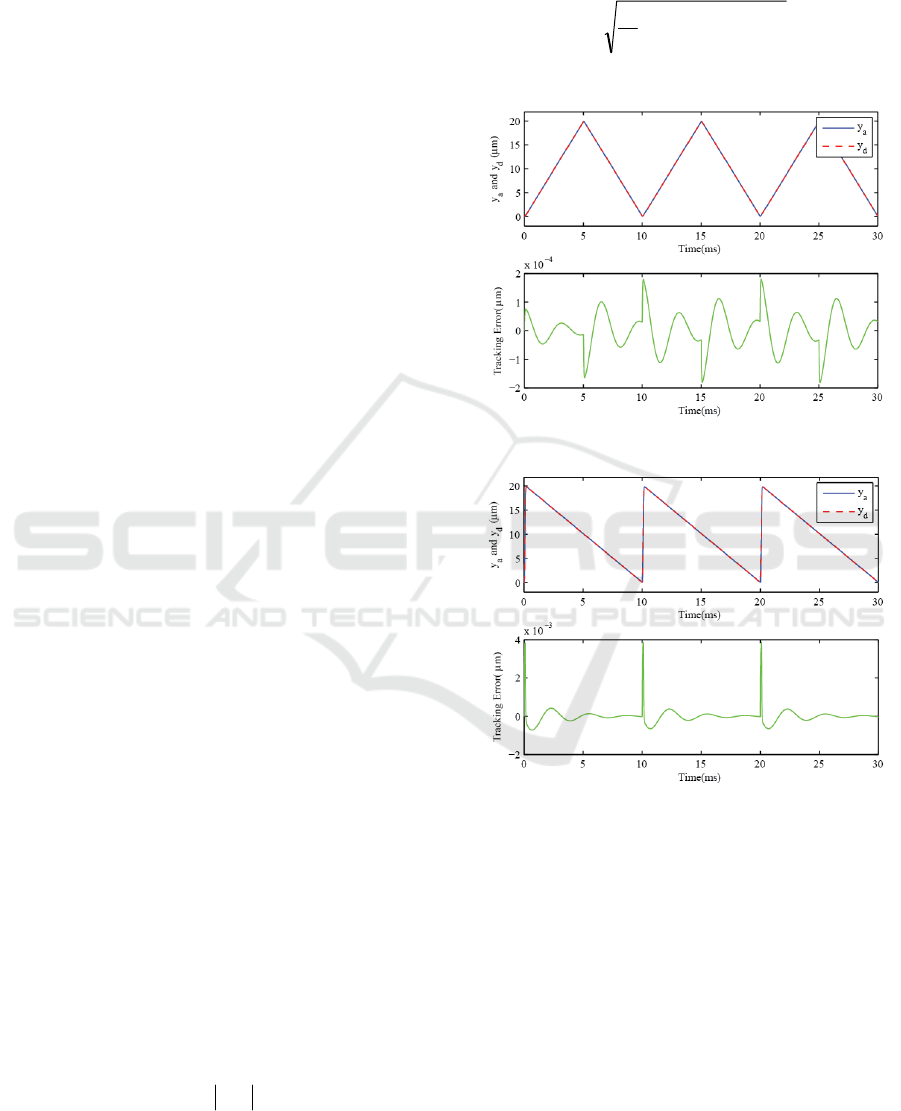
Figure 5: Block diagram used for obtaining the frequency
response of the piezoactuator.
3.2 Transfer Function and Time
Scaling
In this work, the poles, the zeros, and the gain of the
piezoactuator are found experimentally and the
experimental result from the frequency response
shows that the model is composed of 6 poles and 4
zeros in the frequency range of 0 to 1000 Hz.
The poles are located in the complex s-plane at
=
⎥
⎥
⎥
⎦
⎤
⎢
⎢
⎢
⎣
⎡
65
43
21
,
,
,
pp
pp
pp
⎥
⎥
⎥
⎦
⎤
⎢
⎢
⎢
⎣
⎡
±
±
±
5361.0i 65.9-
4149.2i 169.4-
1952.7i 346.8-
(1)
The zeros are located in the complex s-plane at
=
⎥
⎦
⎤
⎢
⎣
⎡
43
21
,
,
zz
zz
⎥
⎦
⎤
⎢
⎣
⎡
±
±
5397.6i 49.7-
4027.3i 159.6-
(2)
The constant gain is
K = 1.1879x 10
7
(3)
The poles and the zeros specify and define the
properties of the transfer function, thus describing
the input-output system dynamics. The poles, the
zeros, and the gain K all together completely provide
a full description of the system and characterize the
system dynamics and the response.
The transfer function can now be constructed by
using the poles, the zeros, as well as the gain, and
the resulting transfer function
)(sG
is found to be of
the form.
=)(sG
)10(58.4)10(03.5)10(164.1
)10(395.5)10(973.4)10(188.1
3
1047536
2143947
ssss
sss
+++
+
++
)10(95.1)10(911.3)10(851.6
)10(622.5)10(297.1
...
2117214
2117
++
+
ss
s
(4)
The DC gain of the system in dB is equal to
20log
10
(5.622x10
21
/1.95x10
21
) = 9.20 dB.
The inspection of Eq.(4) indicates that the system
response is very fast with the settling time in
milliseconds. To avoid numerical problems with
simulations in MATLAB, the time unit needs to be
changed from second to millisecond. To do this,
each variable, s, in the transfer function in Eq.(4 ) is
replaced by 1000s ,and the new transfer function
)(sG
ms
in terms of millisecond is obtained as
=)(sG
ms
...
8.453.50164.1
5.539973.488.11
3456
234
s
s
s
s
sss
+++
+++
(5)
19501.3911.685
56227.129
...
2
++
+
s
s
s
The s variable in the new transfer function in Eq.(5)
has the unit in radian/millisecond. In MATLAB, the
time axis must therefore be rescaled to millisecond.
The Bode diagram that represents the frequency
response of the piezoactuator is plotted by using
)(sG
ms
and illustrated in Fig. 6.
Figure 6: Bode diagram of the piezoactuator.
In this work, the sixth-order model of the
actuator is decomposed into three modes of second-
order systems by using the parallel state space
realization method, shown in Fig.7 so that
robustness can be investigated by providing each
mode with variations in the natural frequency and
the damping ratio.
Figure 7: Diagram for parallel state space realization, an
approach to decoupling the modes of oscillations.
Tracking of High-speed, Non-smooth and Microscale-amplitude Wave Trajectories
501

To find the state space representation by the
parallel state space realization method, the transfer
function can be rewritten in the form of partial
fractions.
...
)(
)(
4
4
3
3
2
2
1
1
+
−
+
−
+
−
+
−
=
ps
r
ps
r
ps
r
ps
r
su
sy
(6)
s
k
ps
r
ps
r
+
−
+
−
+
6
6
5
5
...
where
1
r
,
2
r
,…
6
r
are the residues,
1
p
,
2
p
,…
6
p
are the poles of the system, and
s
k
is the direct term.
The direct term is equal to zero for a strictly
proper transfer function. The poles located at
=
s
1
p
,
2
p
, …,
6
p
are shown in Eq.(1), and it follows
that
)()()(
)(
)(
)(
3,2,1,
sGsGsG
su
sy
sG
msmsmsms
++==
(7)
Where
),(
1,
sG
ms
),(
2,
sG
ms
and
)(
3,
sG
ms
are obtained
as follows.
9344.36938.0
1660.110511.0
)(
2
1,
++
+−
=
ss
s
sG
ms
for mode 1
2312.173388.0
8986.00397.0
)(
2
2,
++
+
=
ss
s
sG
ms
for mode 2
7637.281315.0
2050.00114.0
)(
2
3,
++
−
=
ss
s
sG
ms
for mode 3
Now, the system is decoupled to three modes, and
each mode is represented by a second-order transfer
function. The system in Eq.(7) represents the
original system described by Eq.(5) and preserves
the original system response characteristics.
A second-order system possesses a pair of
complex conjugate poles and the pole location
determines the natural frequency and the damping
ratio. For a second-order system, the location of the
poles
21
, ss
is related to the natural frequency
n
ω
and the damping ratio
ζ
by
2
21
1, ζωζω −±−=
nn
iss
(8)
From the pole locations and Eq.(8) above, the
natural frequency
n
ω
and the damping ratio
ζ
for
each mode of vibration can be found and shown in
Table 1. It is noted that the system is stable since all
the poles have a negative real part, and the mode
number is determined by realizing that the higher
mode number will have a greater natural frequency.
Table 1: Pole location, natural frequency and damping
ratio for each mode.
Pole Location
(Hz)
n
ω
ζ
Mode
1952.7i -346.8
1
+=p
315.65 0.175 1
1952.7i -346.8
2
−=p
315.65 0.175 1
4149.2i -169.4
3
+=p
660.92 0.041 2
4149.2i -169.4
4
−=p
660.92 0.041 2
5361.0i -65.9
5
+=p
853.29 0.012 3
i0.5361 -65.9
6
−=p
853.29 0.012 3
4 CONTROL SCHEME
The notions and the developments of inversion-
based control have attracted researchers in the field
and have been around for more than four decades.
The early and remarkable works on inversion-based
approach were presented by Silverman (1969) and
Hirschorn (1979). Later on, many developments and
contributions were made by means of inversion-
based control, or feedforward control methods such
as the works by Peng et al., (1993), Meckl et al.,
(1994), Piazzi et al., (2001), Devasia (2002), Dunne
et al., (2011), Yang et al., (2011) and Boekfah et al.,
(2016). The standard inversion control theory is
based on a known or pre-described trajectory.
In this work, the trajectories are prescribed or
known a priori and the system is a minimum phase
type and is stable. The inversion-based control
approach is hence suited and proposed for tracking
the desired trajectories.
4.1 State Space Representation
It is well known that for a linear time-invariant
system (LTI system), the plant dynamics can be
represented by the state equation of the form.
)()()( tButAxtx +=

(9)
and the output equation of the form.
)()()( tDutCxty +=
(10)
For a strictly proper system such as the case here, D
is equal to zero.
Now
),(
1,
sG
ms
),(
2,
sG
ms
and
)(
3,
sG
ms
in Eq.(7)
can be cast into the state space form of Eq. (9) and
Eq. (10), and matrices A, B, C, and D are as follows.
ICINCO 2016 - 13th International Conference on Informatics in Control, Automation and Robotics
502

⎥
⎥
⎥
⎥
⎥
⎥
⎥
⎥
⎦
⎤
⎢
⎢
⎢
⎢
⎢
⎢
⎢
⎢
⎣
⎡
−−
−−
−−
=
1315.07637.280000
100000
003388.02312.1700
001000
00006938.09344.3
000010
A
⎥
⎥
⎥
⎥
⎥
⎥
⎥
⎥
⎦
⎤
⎢
⎢
⎢
⎢
⎢
⎢
⎢
⎢
⎣
⎡
=
1
0
1
0
1
0
B
[] 0114.02050.00397.08986.00511.0166.11 −−=C
0=D
4.2 Inversion-based Control Approach
The relative degree, r, of the system is defined by
the difference between the number of poles and the
number of zeros. For the model governed by Eq.(5),
the relative degree is the number of poles minus the
number of zeros , or 6 - 4 = 2.
The full order inverse can lead to a
computational drift due to numerical errors in the
simulation software. To avoid the computational
numerical problem, the reduced order inverse
approach is to be used to find the inverse input, as in
the work by Boekfah et al., (2016).
To determine the inverse input in the inversion-
based method, it is necessary to take the rth time
derivative so that the input appears, i.e.,
)()(
)(
1
tBuCAtxCA
dt
tyd
rr
r
r
−
+=
(11)
)()( tuBtxA
yy
+=
The inverse input
inv
u
required to track a
sufficiently smooth trajectory y is determined from
Eq.(11),i.e.,
⎟
⎟
⎠
⎞
⎜
⎜
⎝
⎛
−=
−
)(
)(
)(
1
txA
dt
tyd
Btu
y
r
r
yinv
(12)
In the reduced order inverse, some components of
the state are known when the desired output,
(.)
d
y
,
and its time derivatives are defined. In particular, the
following coordinate transformation can be made.
)(...)(
)(
)(
...
)(
)(
)(
)(
)(
)(
1
)1(
)1(
)1(
tx
T
T
tx
tT
CA
CA
C
t
t
t
ty
dt
d
ty
ty
tz
r
d
d
r
r
d
d
⎥
⎥
⎥
⎦
⎤
⎢
⎢
⎢
⎣
⎡
=
⎥
⎥
⎥
⎥
⎥
⎥
⎥
⎥
⎦
⎤
⎢
⎢
⎢
⎢
⎢
⎢
⎢
⎢
⎣
⎡
=
⎥
⎥
⎥
⎦
⎤
⎢
⎢
⎢
⎣
⎡
=
⎥
⎥
⎥
⎥
⎥
⎥
⎥
⎥
⎦
⎤
⎢
⎢
⎢
⎢
⎢
⎢
⎢
⎢
⎣
⎡
=
−
−
−
η
ζ
η
η
ζ
η
……

……

)(tTx=
(13)
where
(.)
d
ζ
is the known portion of the state, and
η
is the unknown portion of the state, and the
bottom portion
η
T
of the coordinate transformation
matrix T is chosen such that the matrix T is
invertible, leading to the inverse transformation, i.e.,
[]
ηζ
η
ζ
η
ζ
11111
)(
−
+
−
=
−−
=
−
=
⎥
⎥
⎦
⎤
⎢
⎢
⎣
⎡
⎥
⎥
⎦
⎤
⎢
⎢
⎣
⎡
r
T
l
T
r
T
l
TTtx ……
(14)
By taking the time derivative of
η
in Eq.(13) and
using the state equation in Eq.(9),the inverse input in
Eq.(12) can be rewritten as the output of
η
in the
following inverse system.
))()(()()( tButAxTtxTt +==
ηη
η


(15)
Now the state
)(tx
in Eq.(14) can be used in Eq.(15)
to obtain the inverse system.
)()()( tYBtAt
dinvinvinv
+=
η
η

(16)
)()()( tYDtCtu
dinvinvinv
+=
η
(17)
where
η
is termed as the internal state, and
11
)]([
−−
−=
ryyinv
TABBATA
η
])]([[
111 −−−
−=
ylyyinv
BBTTABBATB
ηη

11 −−
−=
ryyinv
TABC
][
111 −−−
−=
ylyinv
BTABD 
⎥
⎦
⎤
⎢
⎣
⎡
=
)(
)(
)(
)(
ty
t
tY
r
d
d
d
ζ
For this particular work of the relative degree
r =2,
there are therefore four more states to be chosen, and
⎥
⎥
⎥
⎥
⎦
⎤
⎢
⎢
⎢
⎢
⎣
⎡
=
6
5
4
3
)(
x
x
x
x
t η
can be chosen.
where
Tracking of High-speed, Non-smooth and Microscale-amplitude Wave Trajectories
503

CAACAA
r
y
==
CABBCAB
r
y
==
−1
⎥
⎥
⎥
⎦
⎤
⎢
⎢
⎢
⎣
⎡
=
η
ζ
T
T
T ...
)(...)(
...
)(
...
)(
)(
...
)( tx
T
T
tx
T
CA
C
t
t
t
y
y
tz
d
d
d
⎥
⎥
⎥
⎦
⎤
⎢
⎢
⎢
⎣
⎡
=
⎥
⎥
⎥
⎥
⎥
⎦
⎤
⎢
⎢
⎢
⎢
⎢
⎣
⎡
=
⎥
⎥
⎥
⎦
⎤
⎢
⎢
⎢
⎣
⎡
=
⎥
⎥
⎥
⎥
⎦
⎤
⎢
⎢
⎢
⎢
⎣
⎡
=
η
ζ
η
η
ζ
η

and the matrix
T is
⎥
⎥
⎥
⎥
⎥
⎥
⎥
⎥
⎦
⎤
⎢
⎢
⎢
⎢
⎢
⎢
⎢
⎢
⎣
⎡
−−−
−−
=
100000
010000
001000
000100
2065.03279.08852.06841.0201.112011.0
0114.02050.00397.08986.00511.0166.11
T
The tracking can now be simulated in MATLAB
computing software.
5 RESULTS AND DISCUSSIONS
With the initial conditions of being zeros for all the
states at time
t = 0, the tracking results are illustrated
in Fig.8 and Fig.9.
5.1 Quantifying Thetracking Errors
To measure the performance of the tracking, the
error
E(t) of tracking, or tracking error can be
defined as
)()()( tytytE
da
−=
(18)
where
)(ty
a
is the actual trajectory output and
)(ty
d
is the desired trajectory output.
Eq.(18) defines an error for each point of time (
t)
and the error for each point of time is plotted along
with the trajectory outputs in Fig. 8 and Fig.9.
Another quantification of tracking performance
that can be used to evaluate the tracking is the
maximum tracking error
max
E
and the maximum
tracking error is given by
)(max
max
tEE =
(19)
To evaluate the overall tracking performance for the
entire tracking time of 30 milliseconds, the root
mean square error (RMSE) can also be used as an
index of the tracking performance, and the root
mean square error is defined as
∑
−=
=
N
i
da
tyty
N
RMSE
1
2
))()((
1
(20)
where N is the number of the data points.
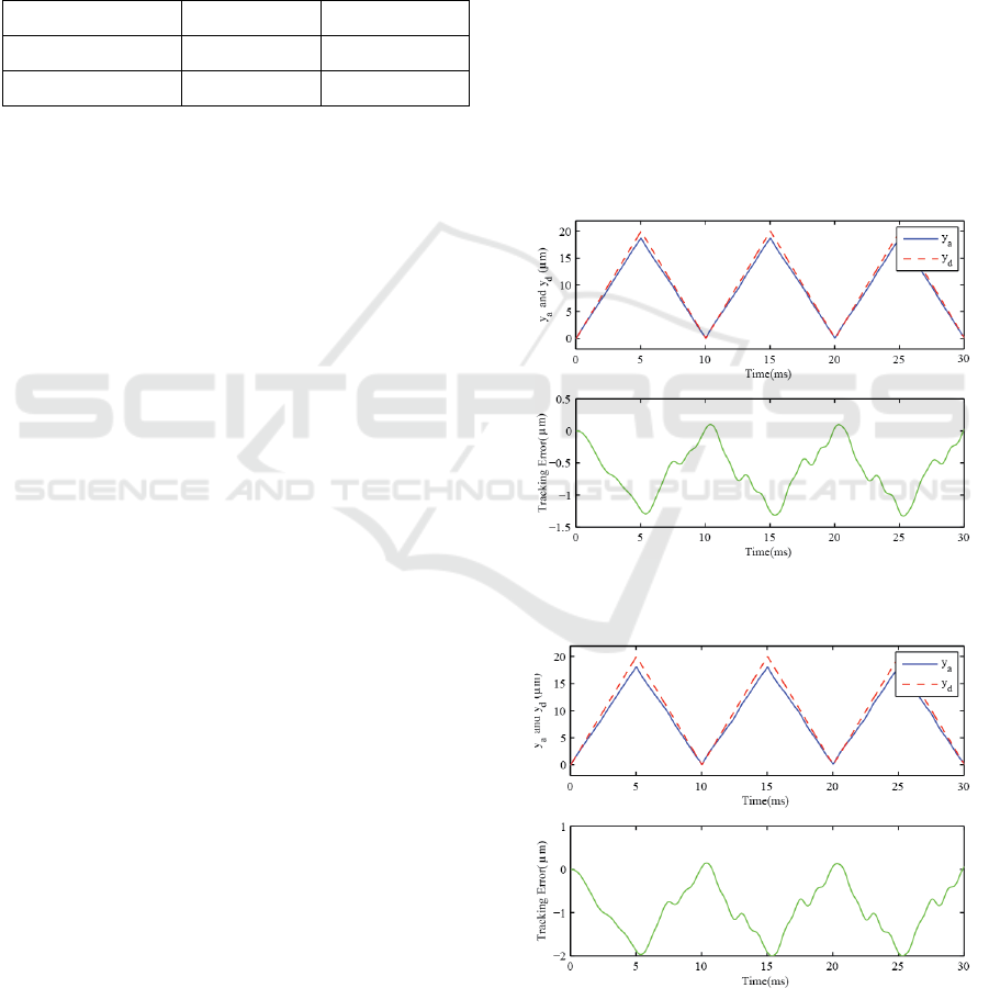
Figure 8: Tracking results for the triangle wave trajectory.
Figure 9: Tracking results for the sawtooth wave
trajectory.
5.2 Tracking Performance
From Fig.8 and Fig.9, it can be seen that the tracking
error tends to reach a maximum value at the
turnarounds of the waves. Table 2 shows very small
values of the
max
E
and the RMSE values of tracking
the triangle wave and the saw tooth wave and
indicates very good tracking performances. In
particular,
max
E
values are very small, compared to
the wave amplitude of 10
m
μ
i.e.,
4
1081.1
−
×
m
μ
for
the triangle wave and
3
1087.3
−
×
m
μ
for the
sawtooth wave. This reports that the tracking
ICINCO 2016 - 13th International Conference on Informatics in Control, Automation and Robotics
504

performance is very good. Table 2 also indicates that
tracking the saw tooth wave (with sharper
turnarounds at the corner, compared to the triangle
wave) yields larger values of the
max
E
and the RMSE
values, compared to tracking the triangle wave. In
other words, tracking of the sawtooth wave is more
difficult than that of the triangle wave.
Table 2: Maximum Error (
max
E
) and Root Mean Square
Error (RMSE).
Wave Type
max
E
)( m μ
RMSE
)( m μ
Triangle
4
1081.1
−
×
5
1050.6
−
×
Sawtooth
3
1087.3
−
×
4
1011.4
−
×
6 ROBUSTNESS OF TRACKING
To delve into the robustness against unmodeled
dynamics, modeling error, or disturbance, for this
particular study, it is
assumed that the natural
frequency
n
ω
and the damping ratio
ζ
are
increased by some percentage.
There are four cases that are investigated for
each trajectory for the study of robustness.
Case [1]:
n
ω
and
ζ
are not changed and their
numerical values are shown in Table 1.The study of
this case was completed in Section 5.
The plots were shown in Fig.8 for the triangle case
and in Fig.9 for the sawtooth case. The tracking
errors were quantified and shown in Table 2. This is
a reference case for the other three cases.
Case [2]:
n
ω
and
ζ
are increased by 3.2 %.
The plots are shown in Fig. 10 for the triangle case
and in Fig.13 for the sawtooth case.
Case [3]:
n
ω
and
ζ
are increased by 5.0 %.
The plots are shown in Fig.11 for the triangle case
and in Fig.14 for the sawtooth case.
Case [4]:
n
ω
and
ζ
are increased by 10.0 %.
The plots are shown in Fig.12 for the triangle case
and in Fig.15 for the sawtooth case.
For all cases, the tracking errors are quantified
and shown in Table 3 for the case of the triangle
trajectory and Table 4 for the case of the sawtooth
trajectory.
From Fig.10 to Fig.15, Table 3 and Table 4, it is
observed that
1.
E
max
is still less than 10% of the peak to peak
amplitude of 20 micron if the increases in the
natural frequency and the damping ratio are less
than 5% for the triangle trajectory, and E
max
is
still less than 10% of the peak to peak amplitude
of 20 micron if the increases in the natural
frequency and the damping ratio are less than 3.2
% for the sawtooth trajectory.
2.
max
E
and RMSE increase as the percentage of
change in the natural frequency and the damping
ratio is increased.
3.
The tracking is quite sensitive to the change in
the natural frequency and the damping ratio.
Particularly, if the increases by 10%, the tracking
gets worse.
4.
The maximum error tends to occur at the sharp
corner of the trajectories.
5.
The actual trajectory of the sawtooth oscillates
obviously if there are changes in the natural
frequency and the damping ratio.
Figure 10: Tracking results for the triangle wave trajectory
in case [2].
Figure 11: Tracking results for the triangle wave trajectory
in case [3].
Tracking of High-speed, Non-smooth and Microscale-amplitude Wave Trajectories
505

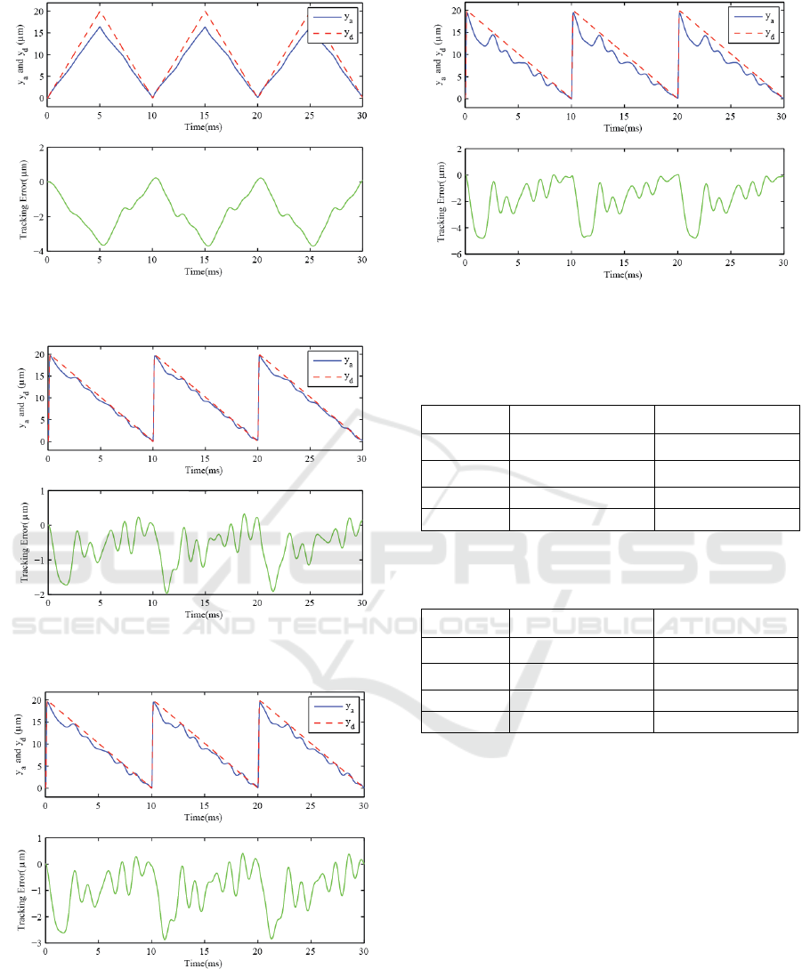
Figure 12: Tracking results for the triangle wave trajectory
in case [4].
Figure 13: Tracking results for the sawtooth wave
trajectory in case [2].
Figure 14: Tracking results for the sawtooth wave
trajectory in case [3].
Figure 15: Tracking results for the sawtooth wave
trajectory in case [4].
Table 3: Maximum Error (
max
E
) and Root Mean Square
Error (RMSE) for triangle trajectory.
Case
max
E )( m
μ
RMSE
)( m
μ
[1]
4
1081.1
−
×
5
1050.6
−
×
[2]
331.1
1
1030.7
−
×
[3]
99.1 11.1
[4]
70.3 06.2
Table 4: Maximum Error (
max
E
) and Root Mean Square
Error (RMSE) for sawtooth trajectory.
Case
max
E )( m
μ
RMSE
)( m
μ
[1]
3
1087.3
−
×
4
1011.4
−
×
[2]
97.1
1
1003.8
−
×
[3]
88.2 22.1
[4]
80.4 21.2
7 CONCLUSIONS
This article presents an inversion-based control
approach to tracking wave trajectories. The
interesting challenge is that the tracking involves the
trajectories that possess a high frequency, a
microscale amplitude, sharp turnarounds at the
corners. The model or transfer function of a
piezoactuator is obtained experimentally from the
frequency response by using a dynamic signal
analyzer. Under the inversion-based control scheme
and the model obtained ,the tracking is simulated in
MATLAB. The main contributions of this work are
to show that (1) the model and the controller achieve
a good tracking performance measured by the root
ICINCO 2016 - 13th International Conference on Informatics in Control, Automation and Robotics
506

mean square error (RMSE) and the maximum error
(E
max
), (2) the maximum error tends to occur at the
sharp corner of the trajectories, (3) tracking the
sawtooth wave yields larger RMSE and E
max
values,
compared to tracking the triangle wave, and (4) in
terms of robustness against modeling error or
unmodeled dynamics, E
max
is still less than 10% of
the peak to peak amplitude of 20 micron if the
increases in the natural frequency and the damping
ratio are less than 5% for the triangle trajectory and
E
max
is still less than 10% of the peak to peak
amplitude of 20 micron if the increases in the
natural frequency and the damping ratio are less than
3.2 % for the sawtooth trajectory.
There is still room for developing the tracking
and improving the tracking performance, in
particular for the robustness against unmodeled
dynamics or disturbances by means of adding a
feedback control to the inversion-based control.
ACKNOWLEDGEMENTS
The author of the article would like to sincerely
thank Assumption University of Thailand for
supporting the research.
REFERENCES
Beschi, M., Dormido, S., Sanchez, J., Visioli, A., and
Yebra, L. J.,(2014) ‘Event-Based PI plus Feedforward
Control Strategies for a Distributed Solar Collector
field’, IEEE Transactions on Control Systems
Technology, Vol. 23, No. 4, July 2014,pp. 1615–1622.
Boekfah, A., and Devasia, S.,(2016) ‘Output-Boundary
Regulation Using Event-Based Feedforward for
Nonminimum-Phase Systems’, IEEE Transactions on
Control Systems Technology, Vol.24,No.1, January
2016, pp265-275.
Devasia, S., (2002). ‘Should Model-Based Inverse Inputs
Be Used as Feedforward Under Plant Uncertainty?’,
IEEE Transactions on Automatic Control, Vol.47,
No.11, November 2002,pp1865-1871.
Dunne, F., Pao, L. Y., Wright, A. D., Jonkman, B., and
Kelley, N.,(2011) ‘Adding Feedforward Blade Pitch
Control to Standard Feedback Controllers for Load
Mitigation in Wind Turbines’, Mechatronics, Vol. 21,
No. 4, June 2011, pp. 682–690.
Hirschorn, R. M., (1979). ‘Invertibility of Multivariable
Nonlinear Control Systems’, IEEE Transactions on
Automatic Control, Vol.AC-24, No.6, December
1979,pp855-865.
Kongthon, J., Chung, J.-H., Riley, J., and Devasia,
S.,(2011)‘Dynamics of Cilia-Based Microfluidic
Devices’, ASME Journal of Dynamic Systems,
Measurement and Control,Vol. 133, September
2011,pp.051012-1-051012-11.
Kongthon, J., and Devasia, S., (2013) ‘Iterative Control of
Piezoactuator for Evaluating Biomimetic, Cilia Based
Micromixing’, IEEE/ASME Transactions on
Mechatronics, Vol.18, No. 3, June 2013, pp 944-953.
Kongthon, J., McKay, B.,Iamratanakul, D., Oh, K.,
Chung, J.-H., Riley, J., and Devasia, S.,(2010)
‘Added-Mass Effect in Modeling of Cilia-Based
Devices for Microfluidic Systems’, ASME Journal of
Vibration and Acoustics, Vol.132, No.2, April 2010,
pp.024501–1–024501–7.
Martin, P., Devasia, S., and Paden, B., (1996). ‘A
Different Look at Output Tracking: Control of a
VTOL Aircraft’, Automatica, Vol. 32, No. 1,pp. 01-
107.
Meckl, P. H.,and Kinceler, R.,(1994) ‘Robust Motion
Control of Flexible Systems Using Feedforward
Forcing Functions’, IEEE Transactions on Control
Systems Technology, Vol. 2, No. 3, September
1994,pp. 245–254.
Moallem, M., Kermani, M. R., Patel, R. V., and Ostojic,
M.,(2004) ‘Flexure Control of a Positioning System
Using Piezoelectric Transducers’, IEEE Transactions
on Control Systems Technology., Vol. 12, No.
5,September 2004,pp. 757–762.
Peng, H., and Tomizuka, M., (1993) ‘Preview Control for
Vehicle Lateral Guidance in Highway Automation’,
ASME Journal of Dynamic Systems, Measurement and
Control, Vol. 115, No. 4, December 1993, pp.679–
686.
Piazzi, A., and Visioli, A.,(2001) ‘Optimal Inversion-
Based Control for the Setpoint Regulation of
Nonminimum-Phase Uncertain Scalar Systems’, IEEE
Transactions on Automatic Control,Vol. 46, October
2001, No. 10, pp. 1654–1659.
Silverman, L. M.,(1969) ‘Inversion of Multivariable
Linear Systems’, IEEE Transactions on Automatic
Control, Vol.AC-14,No.3,June 1969,pp270-276.
Yang, X., Garratt, M., and Pota, H., (2011) ‘Flight
Validation of a Feedforward Gust-Attenuation
Controller for an Autonomous Helicopter’, Robotics
and Autonomous Systems, Vol. 59, No. 12, December
2011, pp. 1070–1079.
Tracking of High-speed, Non-smooth and Microscale-amplitude Wave Trajectories
507