A Task Space Approach for Planar Optimal Robot Tube Following

Matthias Oberherber, Hubert Gattringer, Andreas M¨uller and Michael Schachinger

Institute of Robotics, Johannes Kepler University Linz, Altenberger Str. 69, Linz, Austria

Keywords:

Robotics, Optimal Path Planning, Optimal Tube Following, Dynamic Modeling, Polygonal Paths.

Abstract:

The classical optimal path following problem considers the problem of moving optimally along a predeﬁned

geometric path under technological restrictions. In contrast to optimal path following, optimal tube following

allows deviations from the initial path within a predeﬁned tube to reduce cost even more. The present paper

proposes a modern approach that treats this non-convex problem in task space. This novel method also pro-

vides a simple way to derive optimal trajectories withina tube described in terms of polygonal lines. Numerical

examples are presented that allow to compare the proposed method to existing joint space approaches.

1 INTRODUCTION

Intelligent path planning and motions exploiting the

existing hardware in an optimal way are essential for

modern production lines. Nevertheless, it is still com-

mon to use lines as geometric paths and motion pro-

ﬁles like trapezoidal acceleration or minimum jerk to

follow these lines (Siciliano et al., 2009). An im-

provement for tasks with a deﬁned robot motion can

be achieved by the optimal path following problem.

The latter consist in following a given path in short-

est time possible under kinematic and dynamic con-

straints. It is an established approach to divide the

problem into the geometric path planning followed by

a subsequent optimization of the path following tra-

jectory (Bobrow et al., 1985) (Pfeiffer and Johanni,

1987). Nowadays very efﬁcient algorithms are avail-

able to solve this kind of problem like (Pham, 2013;

Reynoso-Mora et al., 2013; Verscheure et al., 2009b).

If only the start and end points are deﬁned, optimal

point-to-point motion planning can be used. In this

course the path is no longer deﬁned ﬁx, it is optimized

under various restrictions. Beside the kinematic and

dynamic restrictions of the robot, also obstacles have

to be considered (Shiller and Dubowsky, 1988). The

optimization can be performed in task space (Rajan,

1985) or joint space (Antonelli et al., 2005). Usu-

ally the calculation times for this kind of problem are

rather high, compared to the execution times.

Often a predeﬁned path do not have to be fol-

lowed exactly, but within a certain surrounding. (De-

brouwere et al., 2014) proposed a method called opti-

mal tube following, where the path can vary within

a predeﬁned tube around an initial path to reduce

the costs compared to the initial path. They solved

the problem by introducing a joint angle parametriza-

tion, tube approximation and optimization of the path

within the tube to reduce execution times.

Robotic tasks are typically given in task space,

why the paths are usually also planed there. Due

to this the approach proposed in the present paper

is based on an optimization of the geometric end-

effector (EE) path. This path is deﬁned via splines,

which provide many useful properties concerning op-

timization. We will give a comparison to the joint

space approach in (Debrouwere et al., 2014). Further

we show how this idea can be extended to achieve op-

timal trajectories starting with polygonal lines as ge-

ometric path, as they are used e.g. in mobile robotics

(Zou et al., 2006; Zaverucha, 2005).

The focus of the present paper lies on time optimal

trajectories. Nevertheless, the proposed approaches

can also be used for other optimality criteria like en-

ergy consumption.

In the course of this paper derivatives with respect

to the path parameter are marked with a prime x

′

time derivatives with a dot ˙x =

. Small bold letters

are used for vectors, capital bold letters for matrices.

The paper is organized as follows: Section 2 starts

with the geometric path planning followed by the

kinematic and dynamic modeling of the robot. The

time-optimal path following problem is introduced in

section 3. Afterwards, the tube restriction is deﬁned in

section 4. The joint space time-optimal tube follow-

ing is brieﬂy introduced in section 5. Our task space

approach is proposed in section 6. In section 7 we

Oberherber, M., Gattr inger, H., Müller, A. and Schachinger, M.

A Task Space Approach for Planar Optimal Robot Tube Following.

DOI: 10.5220/0005980303270334

In Proceedings of the 13th International Conference on Informatics in Control, Automation and Robotics (ICINCO 2016) - Volume 2, pages 327-334

ISBN: 978-989-758-198-4

327

give a comparison between the joint space and task

space approach. Further we present a numerical ex-

ample for an industrial robot to show the approach’s

functionality concerning polygonal initial paths. Fi-

nally, we conclude our paper and give an insight into

future work in section 8.

2 PATH PLANNING AND

MODELING

The following section brieﬂy covers the geometric

path planning, the kinematic and dynamic modeling

of the manipulator. Further, the parametrization of

the Equations of Motion (EoM) along the scalar path

parameter is introduced.

2.1 Geometric Path Planning

Spline functions provide many useful properties like

the convex hull property, local support property, con-

tinuity or the invariance against translation, rotation

and scaling (Piegl and Tiller, 1997). These proper-

ties, and the existence of very fast algorithms for nu-

merically calculations, like de Boor’s algorithm (De-

Boor, 1978), make splines to an interesting tool in the

ﬁelds of robotics. A three-dimensional spline curve,

describing e.g. the EE-position r

of a robot can be

written as

(s) =

∑

l=1

(s), (1)

with the scalar path parameter s = [s

] (s

- be-

gin of the path, s

- end of the path). N

(s) denote

the B-spline basis functions of degree d, while d

are

the control points (CPs). There are different ways

to deﬁne the basis functions as local or global sup-

port functions. Once the path is deﬁned, the deriva-

tives of the path with respect to the path parameter

′

(s),r

′′

(s) can be calculated easily by differentia-

tion of the basis functions. For details we refer to

(DeBoor, 1978) and (Piegl and Tiller, 1997). An ex-

emplary spatial EE-path, deﬁned via splines, is shown

Figure 1.

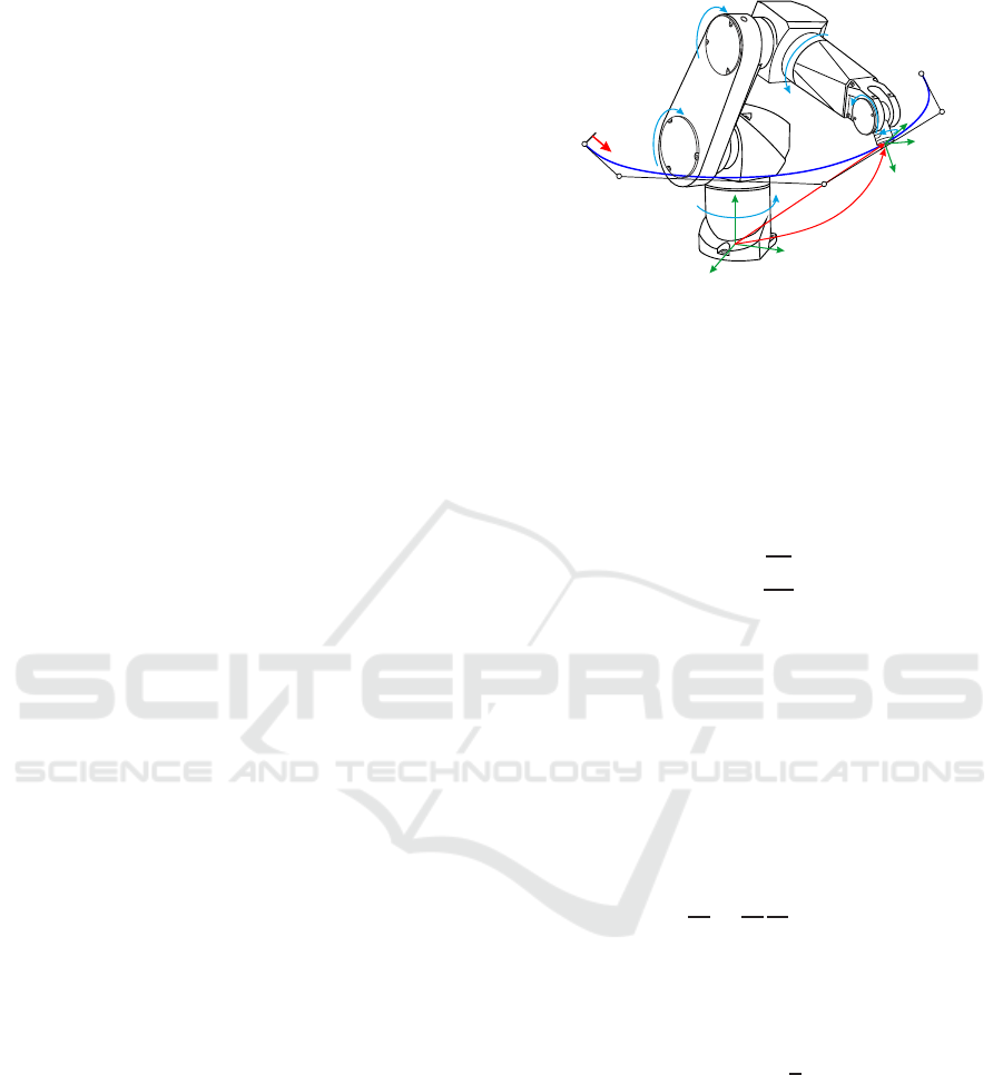
2.2 Kinematic Model

The forward kinematics of a manipulator provides the

EE- coordinates z

(s) = [r

(s),ϕ

(s)] (position r

, orientation ϕ

, e.g. in Cardan angles) as a func-

tion of the joint positions q

q of the robot. Conversely,

the inverse kinematicsq

q(s) = f

−1

(s)) provides the

joint angles as a function of desired EE - coordinates.

There are different ways to solve the locally, but not

−1

(s)

Figure 1: Six-axis industrial robot with joint positions q

globally unique problem of the inverse kinematics.

We use a numerical approach (Siciliano et al., 2009)

based on the relation





= J

J(q

q, (2)

with the EE - velocities v

, ω

represented in the in-

ertial frame and the geometric Jacobian

J =

∂v

∂

∂ω

∂

. (3)

With the Jacobian and r

′

(s), r

′′

(s), the prime quanti-

ties of the joint angles can be calculated as

′

= J

−1

′

(4)

′′

= J

−1



′′

−J

′



. (5)

Near to singularities the Jacobian gets singular. Due

to this a robust inversion J

= (J

J + δ

−1

used, with the identity matrix I and a damping fac-

tor δ that is only active near to singularities.

Using the chain rule for differentiation

= x

′

˙s (6)

and the identity ¨s = (d˙s/ds)(ds/dt) = ( ˙s

)

′

/2, the

joint velocities and accelerations are

q(s) = q

′

(s)˙s (7)

q(s) = q

′′

(s)˙s

′

(s)(˙s

)

′

. (8)

2.3 Dynamic Model

A dynamic model of the robot is necessary to be able

to include torque constraints in the optimization. It

is also used for simulation purposes. The dynamic

model can be written in form of the EoM as

M(q

q+g

g(q

q) = τ

τ (9)

with the position dependent positive deﬁnite mass

matrix M

M(q

q). Joint angles q

q are the minimal coor-

dinates of the system. The vector g

g(q

q) contains all

ICINCO 2016 - 13th International Conference on Informatics in Control, Automation and Robotics

328

nonlinear terms, like Coriolis-, centrifugal-, friction-,

or gravitational forces. The motor torques are denoted

withτ

τ. We derive the EoM with the help of the Projec-

tion Equation (Bremer, 2008). For the path tracking

problem a representation of the EoM in the parameter

range is necessary, and can be written as

τ = a

a(s) ( ˙s

)

′

b(s) ˙s

c(s) +d

(s)˙s. (10)

A method, based on the Projection Equation, to de-

rive the parameters a

a, b

b, c

c and d

analytically is pro-

posed in (Gattringer et al., 2014). Numerical methods

to derive them are presented in (Johanni, 1988) and

(Geu Flores and Kecskemthy, 2012).

3 PATH FOLLOWING PROBLEM

The time optimal robot path following (PF) problem

regards the problem of generating trajectories that fol-

low predeﬁned EE paths in shortest possible time, tak-

ing into account kinematic and dynamic constraints.

Since the path is deﬁned in the parameter range, the

aim is to calculate an optimal relation t(s) between

time and path parameter. We are looking for optimal

solutions for the cycle time t

of a process. Since this

time is the solution of the optimization, it is a priori

unknown. A change of the integration variable from t

to s leads to

1dt =

˙s(s)

ds. (11)

By introducing the abbreviation z = ˙s

the following

optimization problem in parameter space

min

z(·)

z(s)

ds (12)

s.t.

≤ q

′

(s)

z(s) ≤

≤ q

′′

(s)z(s)+

′

(s)z

′

(s) ≤

≤ a

a(s)z

′

(s) +b

b(s)z(s)+c

c(s) +d

(s)

z(s) ≤ τ

τ.

has to be solved. It is assumed that the joint velocity

restrictions

q, joint acceleration restrictions

q and

torque restrictions τ

, τ

τ are constant along the path.

There exist several different approaches to solve

the classical path following problem. In the 1980’s

(Bobrow et al., 1985) proposed a method based on nu-

merical integration and the search of switching points

in the phase plane, while (Shin and McKay, 1986)

used a dynamic programming approach to solve this

kind of problem. Current works in this research ﬁeld

are for example an online log-barrier optimization

(Verscheure et al., 2009b), or a Second Order Cone

Program (SOCP) reformulation of the problem (Ver-

scheure et al., 2009a). These approaches make use of

a convex formulation of the optimization problems.

Nevertheless, (12) is non-convex, due to the inclu-

sion of viscous friction (parameter d

). (Reynoso-

Mora et al., 2013) proposed a method called convex-

relaxation, that empowers them to reformulate the op-

timization as a SOCP anyway.

4 TUBE-RESTRICTION

The tube should constrain the EE-position within a

deﬁned distance r

) to the initial path. Debreuwere

et al. proposed different ways to approximate the

tube. They show, that a linear approximation is com-

putationally more expensive than a quadratic approx-

imation, see Figure 2. In this paper we will use the

quadratic approximation, deﬁned as

= {r

)| (13)

) −r

E,0

))

) −r

E,0

)) ≤ r

)



where C

is the deﬁned space of the tube. The better

performance of the quadratic approximation goes in

contrast with a higher deviation of the approximated

to the original tube. An approximation of the tube

is necessary to allow a tangential relocation of a dis-

crete path point r

) against the initial path r

E,0

see Figure 2. For a detailed explanation of the tube

deﬁnitions we refer to (Debrouwere et al., 2014).

i−1

i+1

)

Figure 2: Quadratic approximation of the tube with the ini-

tial path r

E,0

(s) in black and a modiﬁed path r

(s) in blue.

5 JOINT SPACE APPROACH

(Debrouwere et al., 2014) solves the time optimal PF

problem in joint space, with the joint anglesq

q ∈ R

DOF

as minimal coordinates. These are parametrized along

the path within an upper

q and a lower q

q boundary

using a parameter 0 ≤ λ

λ(s) ≤ 1. Thus, they can be

written as

q(s) = λ

λ(s)q

q(s) + (1−λ

λ(s))q

q(s). (14)

Parameter λ

λ(s) = [λ

(s),... ,λ

DOF

(s)]

can be de-

ﬁned as a spline curve with k

CPs γ

γ. These CPs rep-

resent the optimization variables and the optimization

A Task Space Approach for Planar Optimal Robot Tube Following

329

problem can be written as

min

z(·),γ

z(s)

ds (15)

s.t.

≤ q

′

(s)

z(s) ≤

≤ q

′′

(s)z(s)+

′

(s)z

′

(s) ≤

≤ a

a(s)z

′

(s) +b

b(s)z(s)+c

c(s) +d

(s)

z(s) ≤ τ

0 ≤ λ

λ(s) ≤ 1

(λ

λ(s)) ∈ C

) = r

E,B

) = r

E,E

The last two equality constraints indicate that the start

point (r

E,B

) and end point r

E,E

of the path are ﬁxed.

6 TASK SPACE APPROACH

The following section introduces the task space ap-

proach. The discussion is limited to planar paths.

First the method for general planar paths is intro-

duced. Following, this section shows how this ap-

proach can be used to deriveoptimal trajectories when

the initial path is described in terms of polygonal

lines.

6.1 General Solution Strategy

The solution strategy of the proposed task space ap-

proach is based on a separation of path planning and

the calculation of an optimal motion proﬁle. The

idea is similar to the one proposed in (Rajan, 1985).

First an initial path for the EE of the robot r

E,0

(s) is

planned via the CPs D

D = [d

,.. . ,d

]

using (1).

A time optimal solution for this PF problem is calcu-

lated. In a next step, a path optimization algorithm in

the sense of variation of the CPs is used to get even

faster overall trajectories. Therefore, with the new

CPs, a new EE-path is calculated and again a time

optimal PF problem for this path is solved. This is

repeated till convergence (no further improvement of

the execution time t

) is achieved.

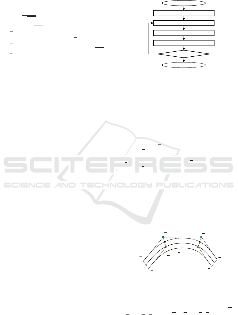
Figure 3 shows a ﬂow-chart of this two-stage op-

timization strategy. An advantage of this method is,

that, depending on the restrictions that have to be con-

sidered, any of the consisting and well tested time op-

timal PF-algorithms like (Bobrow et al., 1985), (Shin

and McKay, 1986), (Verscheure et al., 2009b), (Ver-

scheure et al., 2009a), (Reynoso-Mora et al., 2013),

(Pham, 2013) can be used. The choice of the path op-

timization algorithm is not easy since the problem is

non-convex.

initial path

time optimal PF-optimization

path-optimization (optimize CPs)

calculate new path

convergence?

yes

E,0

optimal trajectory

Figure 3: Solution strategy for the multistage optimization.

6.2 Task Space Approach for Planar

Spline Paths

The following procedure can not only be used for pla-

nar robots, but also for multi-axis robots, when the

EE-path is deﬁned within a plane. In this plane the

path, as well as the tube boundaries can be repre-

sented by splines. The CP locations can be deﬁned

as a convex combination

= d

(1− α

) for j = 1.. .n

− 1. (16)

of the bounding CPs d

and d

of the tube curves

and r

, as shown in Figure 4. The parameters

0 < α

< 1 represent the optimization variables for

the path optimization. Thus, the optimization prob-

lem for the two-stage approach can be written as

min

J (17)

s.t. 0 < α

< 1 for j = 1.. .n

− 1

(s,α

α) ∈ C

wherein the time optimal PF optimization (12) has to

be solved in every iteration of the path optimization.

E,0

(s)

Figure 4: Task space approach: Planar tube and path.

6.3 Tube Following with Polygonal

Lines

In (16) bounding CPs D

= [d

,.. . ,d

]

and D

D =

[

,.. . ,d

]

are deﬁned. Nevertheless, the tube

restriction (13) has to be considered in the optimiza-

tion problem (17). Now, one may ask how they should

ICINCO 2016 - 13th International Conference on Informatics in Control, Automation and Robotics

330

be deﬁned to guarantee that the resulting curve with

the CPs d

= d

(1− α

) lies within the tube.

Unfortunately it is not straight forward to calculate in-

tersection points of splines (Mørken et al., 2009), and

following it is hard to deﬁne the CPs boundings in a

reasonable way for splines.

But, as mentioned in section 1, the usage of

straight lines with subsequent edge combining is still

a wide spread approach for path planning in industrial

applications nowadays. Also the global path planner

of mobile robots often provide polygonal lines, see

e.g. (Zou et al., 2006). For such cases it is a manage-

able problem to deﬁne the position of the bounding

CPs in a reasonable way. In the course of this section

we will present an approach to achieve optimal trajec-

tories along continuous paths, starting with polygonal

lines surrounded by polygonal tube restrictions.

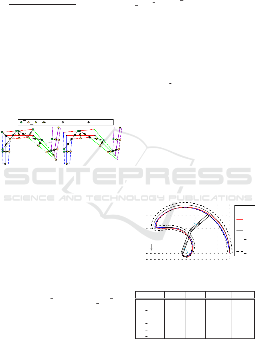
6.3.1 Local Convex Hull Property

To eliminate the possibility of an intersection between

the resulting spline and the tube, we will use the lo-

cal convex hull property, as for example proposed in

(Mørken et al., 2009):

If the unions of all local convex hulls of two

spline curves are disjunct, so are the splines.

If we are able to deﬁne the bounding CPs in a way

that this condition holds, the tube approximation (13)

and the related restriction in the optimization problem

(17) can be omitted.

The local convexhull of a spline curve with degree

d is the smallest convex set, that contains the points

j−d

...d

. In Figure 5 the local convex hulls (exem-

plary for d = 3) of the bounding CPs D

D and D

D are

shown. The presence of multiple CPs let the convex

hull degenerate to lines or points in some cases. The

spline curves r

(s) and r

r(s) deﬁned by D

D and D

D lie

within the union of the local convex hulls. If an in-

tersection between these two curves can be excluded,

the resulting spline r

(s), whose CPs are calculated

as a convex combination of D

and D

D, lies guaranteed

within ther

(s) andr

r(s) and following within the tube.

234

T,1

T,2

r(s)

T,1

T,2

(s)

Figure 5: Local convex hulls for

r(s) (gray), r

r(s) (yellow).

6.3.2 Control Point Placement

We will use the knowledge from section 6.3.1 to de-

ﬁne the CPs positions in a way that the resulting curve

guaranteed lies within the deﬁned tube. For a reason-

able deﬁnition followingpoints have to be considered:

• The polygonal path is deﬁned by the points p

task space coordinates. The angle between two

lines is denoted as ϕ.

• The combination of two lines is called segment.

Following a path consists of n

lines, respectively

= n

− 1 segments.

• The descriptions ’inner’ and ’outer’ corner refer

to a movement along the path from s

to s

• The local convex hulls of r

r(s) and r

r(s) must not

intersect.

• The necessary number of CPs for one segment de-

pends on the spline degree d.

• No overlaps between CPs are allowed.

• The projected tube lengths l

T,i

and l

T,i

denote the

projection of r

T,i

on r

T,i

and conversely the pro-

jection of

T,i

on r

T,i

, as shown in Figure 6 right.

T,1

T,2

T,3

T,1

T,2

T,3

T0,1

TE,1

Figure 6: Left: Tube distance deﬁnition. Right: polygonal

path with tube restrictions and projected tube lengths.

Algorithm:

For all lines k = 1...n

1. Treat special cases

: For ϕ = π the lines are com-

bined to one, the case ϕ = 0 is excepted. Assum-

ing long lines in comparison to the tube distances

avoids the case that a line lies completely within

the tube of an adjacent line.

2. Deﬁne the tubes

: The tubes are deﬁned as lines

with orthogonal distances to the line r

T0,k

and

T0,k

at the start and r

TE,k

and

TE,k

at the end of

the line as shown in Figure 6 left.

3. Generate the overall tube: Calculate the intersec-

tion points between r

T,k

and r

T,k+1

and also be-

tween r

T,k

and r

T,k+1

. Complete the tube by ex-

trapolating and cutting the particular tubes at in-

tersection points as shown in Figure 6 right.

4. Place CPs at half of projected tube lengths:

Bounding CPs d

are placed at l

T,k

/2,

d at l

T,k

/2.

A Task Space Approach for Planar Optimal Robot Tube Following

331

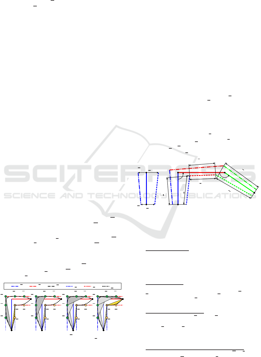
5. Place CPs around the corners: Determine the

connection line between the outer CPs (dotted and

dotdashed in Figure 7 left). If this connection line

lies within the tube (dotdashed), the outer CPs are

also placed there. Otherwise (dotted), the line is

parallel shifted to the inner corner and the outer

CPs are placed at the intersection points of the line

with the outer tube. The inner bounding CPs are

placed at the inner tube corner.

6. Place CPs at the tube corners

: At the tube corners

bounding control points of multiplicity d − 1 are

placed. The number of optimization variables can

be reduced by placing the outer CPs onto the inner

tube corner, as shown in Figure 7 right. Then it

is guaranteed that the path touches the inner tube

corner. This should be an advantage in most cases,

except if the inner corner lies near to a singularity.

j.. j+3

= d

j.. j+1

= d

(α

)

Figure 7: Left: Control point placement for d = 3. Right:

Reduction of optimization variables.

7 EXAMPLES AND RESULTS

At ﬁrst this section gives a comparison of the pro-

posed task space approach with the joint space ap-

proach in terms of a 2D-example deﬁned in (De-

brouwere et al., 2014). Additionally, an example with

polygonal line paths for the industrial robot St¨aubli

RX130L is presented. The following examples are

programmed in Matlab and run on a standard PC with

a 3.4 GHz processor.

7.1 General Planar Paths

The parameters of the 2DOF serial manipulator in

Figure 8 are: l

= l

= 1m, r

s,1

= r

s,2

= 0.5m and

= m

= 1kg. With

τ = [30,10] Nm and τ

τ = −τ

τ, the

motor torque restrictions are given, see (Debrouwere

et al., 2014) for details. The initial joint motion is

deﬁned as

(s) =



−4π(s

− s)

−πs



. (18)

The resulting EE path, see Figure 8, is discretized

into n = 100 pieces. The joint angle restrictions are

(s) =

(s) and

q(s) = 2q

(s), the spline λ

λ(s) is

linear (degree 1). With r

(s) = 0.1(1 − s

) the posi-

tion dependent tube size is deﬁned. For the task space

approach the tube and the EE path have to be approx-

imated by splines, which can be achieved in a satisfy-

ing manner with n

> 10.

In Table 1 a listing of resulting execution and cal-

culation times is given. It should be mentioned that

the calculation times strongly depend on the chosen

path discretization and chosen optimization criteria.

To allow a fair comparison we deﬁned them equally

as much as possible for both approaches. The abbre-

viations are TF TS for tube-following task space, and

TF JS for tube-following in the joint space. These

results show, that both approaches perform nearly

equally for this very simple example. The percent-

age savings in execution time (last column in Table 1)

of the joint space approach are comparable to those

presented in (Debrouwere et al., 2014). Since we use

non-optimized Matlab code for the optimization, cal-

culation times are slightly higher. With the number

of CPs the quality of the solution can be modiﬁed.

The decrease in execution time stands in contrast to a

higher calculation time. A view on Figure 8 shows,

that the optimal paths of the two approaches are quite

different, in spite of the similar execution times. This

is also an evidence on the non-convex characteristic

of the problem. The resulting motor torques normal-

ized on the maximum values as well as the optimal

trends z

opt

(s) are shown in Figure 9.

E,0

E,JS

E,TS

x in m

y in m

−1.5

−1

−0.5

0.5

1.5

0.5

1.5

s,1

s,2

Figure 8: Optimal end-effector paths and tube constraints.

Table 1: Calculation t

CPU

and execution times t

Approach n

, k

in s t

CPU

in s TF/PF

PF - 2.30 0.334 -

TF TS 11 2.20 4.16 4.35%

TF TS 13 2.19 3.81 4.78%

TF TS 15 2.17 5.36 5.65%

TF JS 11 2.17 3.98 5.65%

TF JS 13 2.14 5.46 6.96%

Comparison. Both approaches have their certain

pros and cons. The task space approach does not re-

ICINCO 2016 - 13th International Conference on Informatics in Control, Automation and Robotics

332

0.1

0.2

0.3

0.4

0.5

0.6

0.7

0.8

0.9

0.1

0.2

0.3

0.4

0.5

0.6

0.7

0.8

0.9

−1

z(s)

0.1

0.2

0.3

0.4

0.5 0.6

0.7

0.8

0.9

0.2

0.4

0.6

0.8

Figure 9: Top: Normalized torques τ

τ/τ

τ. Bottom: Optimal

trends z

opt

(s) for all approaches.

quire a joint angle parametrization, which drives up

the optimization time if chosen too big, or addition-

ally restrict the problem if chosen too small. The

number of optimization variables for the path opti-

mization depends on the path length, respectively the

number of chosen CPs for the task space approach

opt

≤ n

−2. While the number of optimization vari-

ables for the path optimization at the joint space ap-

proach also depends on the number of degrees of free-

dom n

opt

= n

DOF

. The necessity of the inverse kine-

matics may be seen as disadvantage of the task space

approach. But, it empowers us to simply include de-

sired EE-orientations ϕ

(s) along the path. While

an additional equality constraint has to be added to

the optimization problem (15) for the joint space ap-

proach to consider a desired EE-orientation.

A big advantage of the task space approach is

that optimal trajectories deﬁned in terms of polygonal

lines as shown in section 6.3 can be derived,where the

tube approximation can be omitted due to an intelli-

gent placement of the CPs, as shown in the following

example.

7.2 Polygonal Lines

The following example is implemented for the indus-

trial robot St¨aubli RX130L in Figure 1. For simplic-

ity, joints q

, q

and q

are locked. In contrast to

the simple example in the section before, several ef-

fects like viscous and Coulomb friction are consid-

ered. The time optimal PF optimization is done with

a dynamic programming approach. Three lines, in the

y - z plane in front of the robot with the points

= [0.75 − 0.5 0.1] m p

= [0.75 − 0.5 1] m

= [0.75 0.5 1] m p

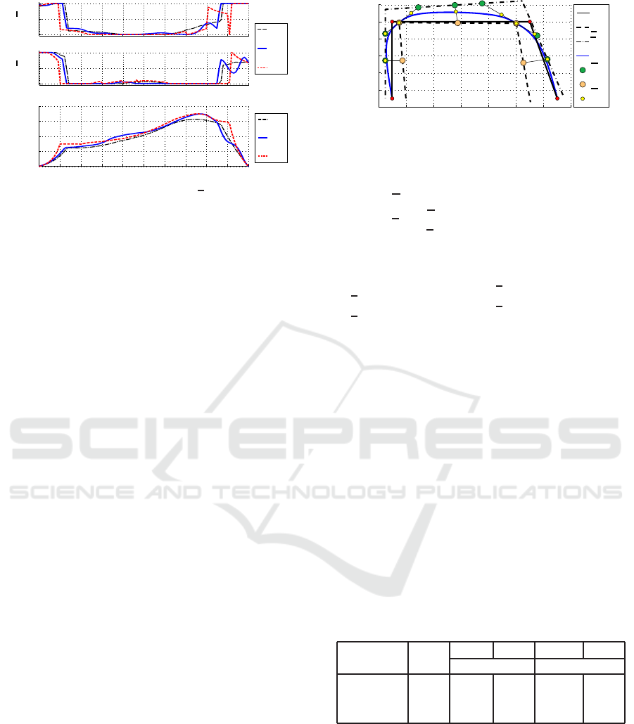
= [0.75 0.7 0.1] m

represent the initial path, shown in Figure 10. This

path is discretized into n = 150 equidistant pieces.

The robot’s hardware restrictions for the joint veloci-

z in m

y in m

E,0

−0.6

−0.4

−0.2

0.2

0.4

0.6

0.8

0.2

0.4

0.6

0.8

1.2

Figure 10: Polygonal path with tube restrictions and result-

ing optimal path with the associated CPs.

ties and motor torques are given as

q = −

= [4.45, 4.45, 5.7]rad/ s (19)

τ = −τ

τ = [9.05, 9.05, 6.4]Nm. (20)

To show some special cases, different tube distances

are chosen for the lines:

= {10, 1, 10} cm, r

= {5, 15, 1} cm

= {5, 2, 20} cm, r

= {5, 25, 5} cm.

The BOBYQA algorithm from NLOPT library (John-

son, 2011) was used via the Matlab interface for path

optimization. For validation purposes several other

algorithms from the NLOPT library were proved, re-

sulting in nearly the same trajectory within differ-

ent calculation times, strongly depending on the dis-

cretization. Resulting joint velocities and torques are

shown in Figure 11. Execution and calculation times

are given in Table 2. Where r

E,0

, indicates the line

path, r

the optimal and r

E,α

the initial path with

= 0.5, j = 1..n

opt

. Fixed corner CPs, as described

in section 6.3.2, reduce the number of optimization

variables from n

opt

= 9 to 7. This inﬂuences not only

the calculation times, but also generates a better ini-

tial solution. The percentage time savings refer to the

time optimal motion along the three lines, where the

robot has to stop after each line.

Table 2: Execution and calculation times.

E,0

E,α

opt

= 9 n

opt

= 7

in s 1.46 1.46 1.14 1.13 1.05

CPU

in s 0.85 0.72 18 0.73 12

save in % — 0 21.7 14.82 22.8

8 CONCLUSIONS

In the present paper we proposed a task space ap-

proach to solve the planar optimal tube following

problem. The focus is on time optimality, neverthe-

less other optimality criteria like energy consump-

tion or path length can also be considered with this

A Task Space Approach for Planar Optimal Robot Tube Following

333

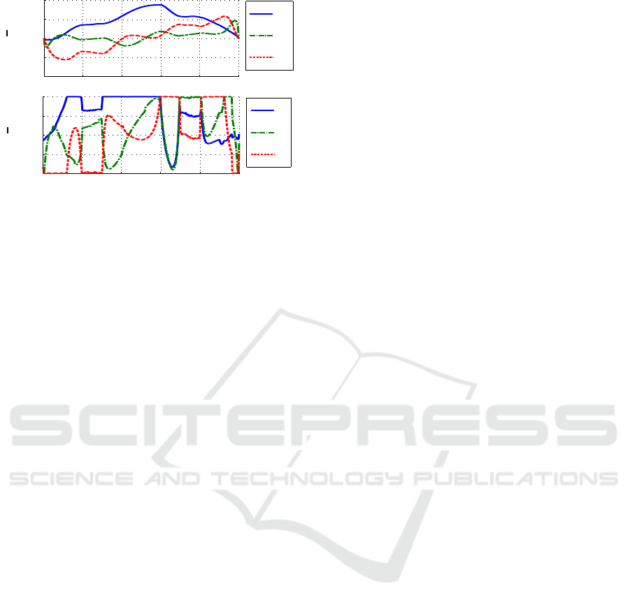
˙q

0.2

0.4

0.6

0.8

−1

−0.5

0.5

τ/

0.2

0.4

0.6

0.8

−1

−0.5

0.5

Figure 11: Top: Normalized joint velocities. Bottom: Nor-

malized motor torques.

method. By means of numerical examples we have

shown that the proposed approach performs nearly

equally to an existing one, with the beneﬁt that opti-

mal trajectories from polygonal paths without an ad-

ditional tube restriction can be derived. Future works

will include among other things further improvements

of the algorithm, an automatism for the tube genera-

tion and the extension to spatial paths.

ACKNOWLEDGEMENTS

This work has been supported by the Linz Center of

Mechatronics (LCM) in the framework of the Aus-

trian COMET-K2 program.

REFERENCES

Antonelli, G., Chiaverini, S., Palladino, M., Gerio, G. P.,

and Renga, G. (2005). Joint space point-to-point mo-

tion planning for robots: An industrial implementa-

tion. In Ztek, P., editor, Proceedings of the 16th IFAC

World Congress.

Bobrow, J. E., Dubowsky, S., and Gibson, J. S. (1985).

Time-optimal control of robotic manipulators along

speciﬁed paths. International Journal Robotics Re-

sarch, 4:3–17.

Bremer, H. (2008). Elastic Multibody Dynamics: A Direct

Ritz Approach. Springer Verlag, Heidelberg.

DeBoor, C. (1978). A practical guide to splines. Springer.

Debrouwere, F., Van Loock, W., Pipeleers, G., and Sw-

evers, J. (2014). Time-optimal tube following for

robotic manipulators. In Advanced Motion Control

(AMC),2014 IEEE 13th International Workshop on,

pages 392–397.

Gattringer, H., Oberherber, M., and Springer, K. (2014).

Extending continuous path trajectories to point-to-

point trajectories by varying intermediate points.

International Journal of Mechanics and Control,

15(01):35–43.

Geu Flores, F. and Kecskemthy, A. (2012). Time-optimal

path palanning along speciﬁed trajectories. In Gat-

tringer, H. and Gerstmayr, J., editors, Multibody Sys-

tem Dynamics, Robotics and Control, pages 1–15.

Johanni, R. (1988). Optimale Bahnplanung bei Industrier-

obotern. Technische Universit¨at M¨unchen.

Johnson, S. G. (2011). The NLopt nonlinear-optimization

package.

Mørken, K., Reimers, M., and Schulz, C. (2009). Com-

puting intersections of planar spline curves using knot

insertion. Comput. Aided Geom. Des., 26(3):351–366.

Pfeiffer, F. and Johanni, R. (1987). A concept for manipula-

tor trajectory planning. IEEE Journal of Robotics and

Automation, 3(2):115 –123.

Pham, Q. (2013). A general, fast, and robust implementa-

tion of the time-optimal path parameterization algo-

rithm. CoRR, abs/1312.6533.

Piegl, L. A. and Tiller, W. (1997). The NURBS book (2. ed.).

Monographs in visual communication. Springer.

Rajan, V. (1985). Minimum time trajectory planning. In

Robotics and Automation. Proceedings. 1985 IEEE

International Conference on, volume 2, pages 759–

764.

Reynoso-Mora, P., Chen, W., and Tomizuka, M. (2013).

On the time-optimal trajectory planning and control of

robotic manipulators along predeﬁned paths. In Amer-

ican Control Conference (ACC), 2013, pages 371–

377.

Shiller, Z. and Dubowsky, S. (1988). Global time optimal

motions of robotic manipulators in the presence of ob-

stacles. In Robotics and Automation, 1988. Proceed-

ings., 1988 IEEE International Conference on, pages

370–375 vol.1.

Shin, K. G. and McKay, N. D. (1986). A dynamic pro-

gramming approach to trajectory planning of robotic

manipulators. Automatic Control, IEEE Transactions

on, 31(6):491–500.

Siciliano, B., Sciavicco, L., Villani, L., and Oriolo, G.

(2009). Robotics - Modelling, Planning and Control.

Advanced Textbooks in Control and Signal Process-

ing series. Springer.

Verscheure, D., Demeulenaere, B., Swevers, J., De Schutter,

J., and Diehl, M. (2009a). Time-optimal path tracking

for robots: A convex optimization approach. Auto-

matic Control, IEEE Transactions on, 54(10):2318–

2327.

Verscheure, D., Diehl, M., De Schutter, J., and Swevers,

J. (2009b). Recursive log-barrier method for on-line

time-optimal robot path tracking. In American Con-

trol Conference, 2009. ACC ’09., pages 4134 –4140.

Zaverucha, G. (2005). Approximating polylines by curved

paths. In Mechatronics and Automation, 2005 IEEE

International Conference, volume 2, pages 758–763

Vol. 2.

Zou, A.-M., Hou, Z.-G., Tan, M., and Liu, D. (2006). Path

planning for mobile robots using straight lines. In Net-

working, Sensing and Control, 2006. ICNSC ’06. Pro-

ceedings of the 2006 IEEE International Conference

on, pages 204–208.

ICINCO 2016 - 13th International Conference on Informatics in Control, Automation and Robotics

334