Application of Trajectory Optimization Method for a Space

Manipulator with Four Degrees of Freedom

Tomasz Rybus

, Karol Seweryn

and Jurek Z. Sąsiadek

Space Research Centre (CBK PAN), Bartycka 18a, Warsaw, Poland

Department of Mechanical and Aerospace Eng., Carleton University, Ottawa, Ontario, Canada

Keywords: Space Robotics, Free-floating Space Manipulator, Trajectory Optimization, On-orbit Servicing.

Abstract: Planned active debris removal and on-orbit servicing missions require capabilities for capturing objects on

Earth’s orbit, e.g., by the use of a manipulator. In this paper we demonstrate the application of a trajectory

optimization algorithm for free-floating satellite-manipulator systems in two cases: a planar system with

2 degrees of freedom manipulator and a spatial system with a manipulator having four degrees of freedom.

For the case with planar system, results of experiments performed on an air-bearing microgravity simulator

are shown. Quadratic norm connected with the power consumption of manipulator motors has been used as

a cost functional that is minimized. Optimal trajectories are compared with straight-line trajectories and it is

shown that the optimization allows reduction of the power use of manipulator motors (for the planar system

30 trajectories based on randomly selected initial and final end-effector positions were analysed and the cost

functional was, on average, reduced by 49.4%). The presented method could be modified by using cost

functional that would, e.g., minimize disturbance on the satellite.

1 INTRODUCTION

Capabilities for capturing objects on Earth’s orbit by

unmanned satellites are required in planned active

debris removal and on-orbit servicing missions.

European Space Agency (ESA) is studying the

concept of active debris removal to prevent

predicted growth of space debris population on Low

Earth Orbit. Studies show that current debris

population is likely to increase due to collisions

between existing space debris (Liou, Johnson, and

Hill, 2010). Thus, removal of large intact objects

from orbit might be necessary in the coming years.

On-orbit servicing missions are proposed to prolong

the operational lifetime of satellites. Repairing

satellite with unmanned servicing vehicle could be

economically feasible (Sullivan and Akin, 2012).

Specific active debris removal and on-orbit servicing

missions have been proposed in recent years, e.g., by

Hausmann et al. (2015). Many of the proposed

mission concepts rely on the use of a manipulator for

performing capture manoeuvre.

Design of a manipulator for orbital operations is

a challenging task, since such manipulators are

complex mechatronic systems that must operate in

space environment and must have a very low mass.

Control of a satellite-manipulator system during

capture manoeuvre is also one of the major

challenges in on-orbit servicing. The motion of the

manipulator influences both the position and the

orientation of the manipulator-equipped satellite.

This effect must be taken into account during

manipulator trajectory planning and control.

Reaction torques and forces induced by the motion

of the manipulator must either be fully compensated

by the guidance, navigation and control subsystem

(GNC) of the satellite or this subsystem must be

switched off during the manoeuvre. In the latter

case, the satellite is in free-floating state (Dubowsky

and Papadopoulos, 1993).

In our study we focus on the subject of end-

effector trajectory planning for a free-floating

manipulator. Methods that allow optimization of

planned trajectory are especially interesting and

several approaches to optimal trajectory planning

and control were developed in the last decade, e.g.,

by Aghili (2008) and Flores-Abad et al. (2014a).

Another benefit of optimization techniques is that

they could also be used to minimize manipulator

disturbances on the manipulator-equipped satellite

(Kaigom, Jung and Rossmann, 2011). The broad

review of on-orbit servicing technologies presented

Rybus, T., Seweryn, K. and S ˛asiadek, J.

Application of Trajectory Optimization Method for a Space Manipulator with Four Degrees of Freedom.

DOI: 10.5220/0005981000920101

In Proceedings of the 13th International Conference on Informatics in Control, Automation and Robotics (ICINCO 2016) - Volume 1, pages 92-101

ISBN: 978-989-758-198-4

by Flores-Abad et al. (2014b) includes a section

devoted to trajectory planning. In our paper we

follow the approach for optimal trajectory planning

that was proposed by Seweryn and Banaszkiewicz

(2008). This approach is based on the Generalized

Jacobian Matrix (GJM), introduced by Umetani and

Yoshida (1989) for systems with zero linear and

angular momentum. Seweryn and Banaszkiewicz

extended GJM for systems with non-zero and not-

conserved linear and angular momentum (e.g., with

additional forces from thrusters acting on the

satellite during the realization of the end-effector

trajectory). They proposed an optimization

algorithm that is based on the calculus of variations.

The cost functional trades off for power use of

motors in the manipulator joints as well as for

additional conditions constraining the end-effector

motion. Rybus, Seweryn and Sąsiadek (2016)

presented several improvements to this algorithm,

the most important being the modification of the

boundary conditions of the optimization problem to

allow imposing constraints for the end-effector

velocity. During the capture manoeuvre the end-

effector velocity at the moment of grasping must

match the velocity of the grasping point on the target

satellite; thus, it is required to define the final end-

effector velocity during the trajectory optimization.

The original algorithm was also extended to include

the time of the manipulator motion as a parameter

that is optimized. As a result, it is possible to

compute the optimal time for the capture

manoeuvre. The trajectory optimization algorithm is

suitable for a general case of a manipulator with n

degrees of freedom, but Rybus, Seweryn and

Sąsiadek (2016) illustrated the presentation of their

algorithm with only a simple example (i.e. a planar

manipulator with 2 degrees of freedom).

In this paper we demonstrate the use of the

aforementioned algorithm for the optimization of

end-effector trajectory of a spatial manipulator with

4 degrees of freedom, mounted on a free-floating

satellite. As torques required to position the end-

effector are much higher than torques needed for

obtaining the desired end-effector orientation, we do

not consider the optimization of end-effector

orientation. In the presented numerical example we

use mass and geometrical properties of the prototype

robotic arm WMS1 LEMUR presented by Seweryn

et al. (2014). WMS1 LEMUR has 7 degrees of

freedom: four joints are responsible for obtaining the

end-effector position (one joint is redundant) and

three joints are responsible for obtaining the end-

effector orientation. In this study we use the

trajectory planning algorithm for the first four joints.

Demonstrating that the optimization method

proposed by Seweryn and Banaszkiewicz (2008) and

extended by Rybus, Seweryn and Sąsiadek (2016)

can be successfully used for a real spatial

manipulator is the main contribution of this paper.

Following Rybus and Seweryn (2015), we also

present the results of an experimental study, in

which trajectory optimization was performed for a

real planar free-floating system with a manipulator

with 2 degrees of freedom. The planar air-bearing

microgravity simulator described by Rybus et al.

(2013) was used for this purpose. In order to assess

the advantages of the optimization algorithm in this

simplified planar case we compared the optimal

trajectory with a straight-line trajectory for 30

randomly selected initial and final positions of the

end-effector.

The paper is organized as follows. In Section 2,

equations describing the dynamics of a free-floating

satellite-manipulator system are presented, while the

trajectory optimization algorithm is shown in

Section 3. Equations contained in these two sections

were earlier presented by Rybus, Seweryn and

Sąsiadek (2016). The results of experiments

performed on the microgravity simulator are shown

in Section 4. Application of the optimization

algorithm for the manipulator with 4 degrees of

freedom is presented in Section 5. Discussion is

presented in Section 6 and the paper concludes with

Section 7.

2 FREE-FLOATING

SATELLITE-MANIPULATOR

SYSTEMS

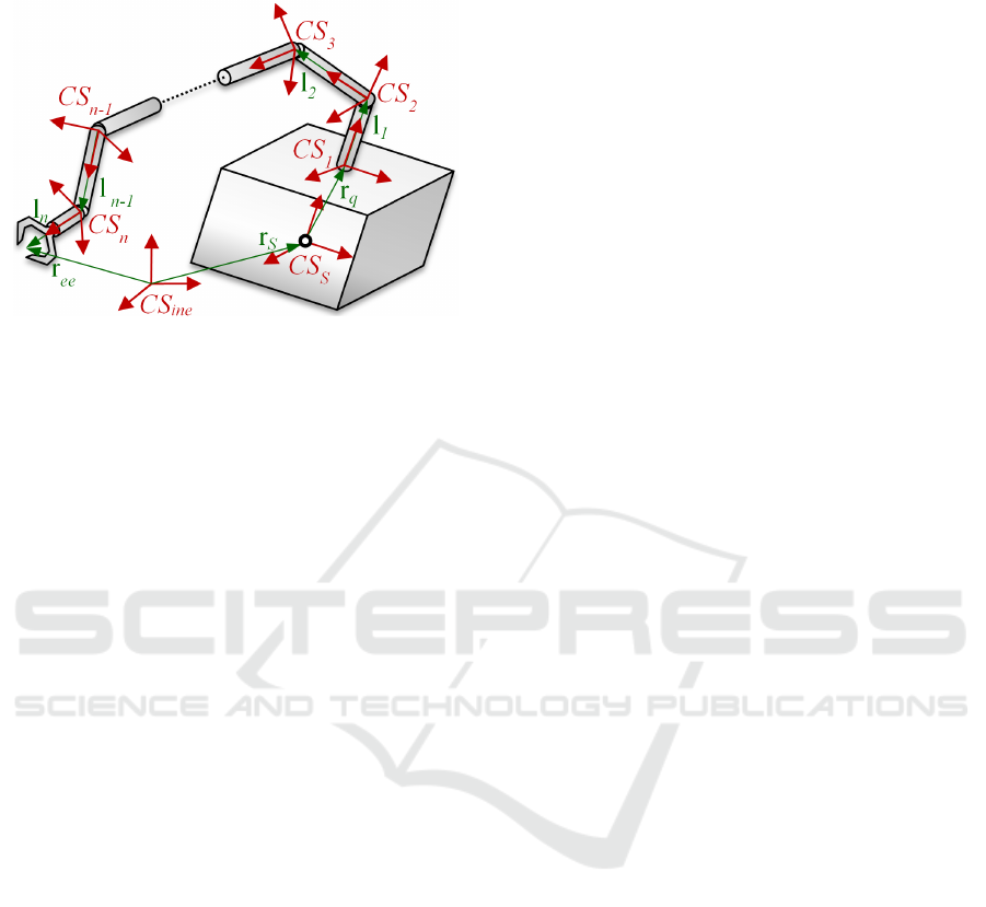
A free-floating satellite equipped with a manipulator

with n degrees of freedom is presented in Fig. 1,

where coordinate systems and selected geometrical

parameters of the satellite-manipulator system are

shown. In this section we follow the approach

presented by Seweryn and Banaszkiewicz (2008)

and by Rybus, Seweryn and Sąsiadek (2016).

All equations are expressed in the inertial

reference frame (denoted as CS

ine

in Fig. 1). The

end-effector position is expressed as:

∑

++=

iqsee

lrrr

(1)

where r

is the position of the satellite center of

mass, r

is the position of the first kinematic pair of

the manipulator with respect to the satellite, and l

Application of Trajectory Optimization Method for a Space Manipulator with Four Degrees of Freedom

the position of the i+1 kinematic pair in respect to

the ith kinematic pair.

Figure 1: A schematic view of the satellite-manipulator

system.

End-effector linear and angular velocities are given

by the following equation:

θJ



⎥

⎦

⎤

⎢

⎣

⎡

⎥

⎦

⎤

⎢

⎣

⎡

(2)

where:

⎥

⎦

⎤

⎢

⎣

⎡

see

(3)

() ( )

⎥

⎦

⎤

⎢

⎣

⎡

−×−×

neenee

rrkrrk



(4)

In the above equations v

and ω

are the linear and

angular velocities of the satellite,



is the n-

dimensional vector containing angular velocities of

the manipulator joints, J

is the Jacobian of the

satellite (6 x 6 matrix), while J

is the standard

Jacobian of a non-space manipulator expressed in

the inertial reference frame (6 x n matrix), I denotes

the identity matrix, 0 denotes the zero matrix,

ee_s

= r

– r

, ~ denotes a matrix which is equivalent

of a vector cross-product, k

and r

are the unit

vector of angular velocity and the position of the ith

kinematic pair, respectively. The angular momentum

of the satellite-manipulator system can be expressed

as:

PrLL ×+=

(5)

where L

is the initial angular momentum of the

system. The momentum P and the angular

momentum of the satellite-manipulator system are

given by the following equation:

⎥

⎦

⎤

⎢

⎣

⎡

⎥

⎦

⎤

⎢

⎣

⎡

⎥

⎦

⎤

⎢

⎣

⎡

×+

θH

PrL



(6)

where:

⎥

⎦

⎤

⎢

⎣

⎡

BrEArB

(7)

⎥

⎦

⎤

⎢

⎣

⎡

DrF

(8)

Here it should be noted that the matrices H

i H

are

influenced not only by the state of the manipulator,

but also by the state of the satellite. The submatrices

A, B, D, E and F are defined as:

⎟

⎠

⎞

⎜

⎝

⎛

∑

(9)

s_q

mm rB

⎟

⎠

⎞

⎜

⎝

⎛

∑

(10)

∑

Tii

(11)

()

∑

++=

siiis

rrIIE

(12)

()

∑

TisiiRii

JrJIF

(13)

where r

s_q

= r

– r

and r

i_s

= r

– r

, m

and I

are the

mass and inertia matrix of the satellite, respectively,

and I

are the mass and inertia matrix of ith

manipulator link, respectively, J

is the translational

component of the manipulator Jacobian J

, while J

is the rotational component of this Jacobian. In a

free-floating system, the linear and the angular

momentum are usually assumed as zero. Such

assumption was taken, e.g., by Dubowsky and

Papadopoulos (1993), Umetani and Yoshida (1989),

and Lindberg, Longman, and Zedd (1993).

However, in the approach introduced by Seweryn

and Banaszkiewicz (2008) and presented herein, the

momentum and angular momentum are not equal to

zero. Instead, in eqn. (6) the momentum and the

angular momentum are described by the time

dependent functions f

and f

defined as:

∫

= dt

and

∫

+= dt

sssam

FrHf

, where F

and H

are forces and torques acting on the satellite. These

could be forces and torques generated by the satellite

ICINCO 2016 - 13th International Conference on Informatics in Control, Automation and Robotics

manoeuvring thrusters or external disturbances (e.g.,

forces and torques resulting from the gravity

gradient).

The end-effector velocity is:

()

θHHJJ



−−

−+

⎥

⎦

⎤

⎢

⎣

⎡

⎥

⎦

⎤

⎢

⎣

⎡

(14)

The following equation relates the angular velocities

of joints with end-effector velocity in the CS

ine

()

⎟

⎠

⎞

⎜

⎝

⎛

⎥

⎦

⎤

⎢

⎣

⎡

−

⎥

⎦

⎤

⎢

⎣

⎡

−=

−

HHJJθ



(15)

The satellite velocity is given by:

⎟

⎠

⎞

⎜

⎝

⎛

−

⎥

⎦

⎤

⎢

⎣

⎡

⎥

⎦

⎤

⎢

⎣

⎡

−

θH



(16)

As in (Seweryn and Banaszkiewicz, 2008) and

(Rybus, Seweryn and Sąsiadek, 2016), we use

Langrangian formalism to derive dynamics

equations for the system. For the considered case of

a system free-floating in space, the potential energy

is neglected. We use the generalized coordinates

(Junkins and Schaub, 1997):

[]

ssp

θΘrq =

(17)

where Θ

is the orientation of the satellite. Following

Seweryn and Banaszkiewicz (2008) we describe the

orientation of the satellite by Euler angles, as their

use is more intuitive and straightforward than the

use of quaternions or orientation matrices. In the

range of motion considered herein, the risk of

obtaining singular configuration is very limited

(there is no tumbling motion of the manipulator-

equipped satellite). The Lagrange equation is:

∂

−

⎟

⎠

⎞

⎜

⎝

⎛

∂



(18)

where T is the kinetic energy of the system

expressed as:

⎥

⎦

⎤

⎢

⎣

⎡

⎥

⎦

⎤

⎢

⎣

⎡

⎥

⎦

⎤

⎢

⎣

⎡

NFD

FEB

DBA



(19)

and Q is the vector of generalized forces:

[]

uHFQ = ,

(20)

where u is the control vector composed of driving

torques in manipulator joints. In eqn. (19) the N

matrix is given by:

()

∑

TiiRii

JJJIJN

(21)

Equation (18) is used to derive the generalized

equations of motion for the satellite-manipulator

system:

(

)

(

)

ppppp

qqqCqqMQ



,+=

(22)

where M denotes the mass matrix expressed as:

()

⎥

⎦

⎤

⎢

⎣

⎡

NFD

FEB

DBA

(23)

while C is the Coriolis Matrix with components

given by:

∑

⎟

⎠

⎞

⎜

⎝

⎛

−=

(24)

where

(

)

pij

m qM∈

and nkji …1,, = .

In eqn. (22) there are no potential forces, as the

considered system is the state of free fall. Equation

(22) can be used to determine the control vector u(

t).

3 TRAJECTORY

OPTIMIZATION

The approach to the end-effector trajectory

optimization that we use in our study was presented

by Seweryn and Banaszkiewicz (2008), with

improvements introduced by Rybus, Seweryn and

Sąsiadek (2016) to enhance the capabilities of the

algorithm. The optimization problem is how to drive

the end-effector from its initial state to the desired

final state while minimizing the optimization

criterion.

The general form of the optimized functional

G is:

() ()

(

)

=tttG

,,uq

() ()

()

() () ()

()

[]

∫

vpvp

dttttttttL

,,,, uqgλuq

(25)

where q

= [q

]

q =

= [λ

]

, λ

and λ

denotes the Lagrange multipliers associated

with q

and q

, respectively, while the function g

describes the direct dynamics of the satellite-

manipulator system:

Application of Trajectory Optimization Method for a Space Manipulator with Four Degrees of Freedom

()

⎥

⎦

⎤

⎢

⎣

⎡

−

⎥

⎦

⎤

⎢

⎣

⎡

−

CqQM



(26)

In eqn. (25)

L is the cost functional to be minimized.

The selection of the appropriate cost functional is

not simple. This selection should be performed by a

control engineer for the specific mission, taking into

account the limitations and conditions defined for

this mission. In papers related to space robotics, a

criterion that assures minimization of changes of the

satellite orientation is most commonly used, e.g., by

Kaigom, Jung and Rossmann (2011), as any

substantial changes of the satellite attitude should be

avoided during the capture manoeuvre. However,

some authors also take into account the power use of

manipulator motors, e.g., Shah et al. (2013). In our

study we follow the approach of Seweryn and

Banaszkiewicz (2008) and we use quadratic norm of

the control input as a cost functional:

(27)

Such a simple cost functional, related to the power

use of manipulator motors, is very common in

automation and robotic. The presented method could

easily be modified by using more complex cost

functional that would allow for achievement of

different goal. The Hamiltonian of the system is

given by:

gλ

LH +=

(28)

The extremum of

G is found for:

∂

(29)

From eqn. (29), the control vector u can be

computed. We define a state vector as:

[]

pvpv

λλqqx =

(30)

and obtain a set of 2(12 + 2

n) differential equations

that minimize the functional

G and satisfy the

boundary conditions:

⎥

⎦

⎤

⎢

⎣

⎡

∂

−

∂

−

⎥

⎦

⎤

⎢

⎣

⎡



(31)

A Boundary Value Problem (BVP) is formulated

and a set of eqn. (31) is solved with 2(12 + 2

boundary conditions and 12 additional equations,

which must be satisfied by the BVP solver. The

initial state of the system (q

at the initial time t

) is

determined by the first 12 + 2

n boundary conditions,

while the values of Lagrange multipliers at the final

time

are determined by another 12 + 2n equations.

These Lagrange multipliers are calculated from the

following equation:

()

fvp

⎟

⎠

⎞

⎜

⎝

⎛

∂

vλ

(32)

Where the function ψ describes the final desired

state of the end-effector (ψ = [r

]

Additional 12 parameters v are determined by the

algorithm to satisfy equations for ψ.

4 APPLICATION OF THE

OPTIMIZATION ALGORITHM

FOR A PLANAR

MANIPULATOR WITH 2

DEGREES OF FREEDOM

To demonstrate the trajectory optimization

algorithm, we performed an experiment on the

planar air-bearing microgravity simulator described

by Rybus et al. (2013). This simulator is a test-bed

that allows for experimental validation of trajectory

planning and control algorithms for free-floating

satellite-manipulator systems. In this test-bed, a

model of a satellite-manipulator system is mounted

on planar air-bearings that allow almost frictionless

motion on a 2x3

granite plate. Thus, microgravity

conditions are simulated in two dimensions.

Currently, a satellite model equipped with a

manipulator with 2 degrees of freedom is operated

on this testbed. Its parameters are summarized in

Tab. 1. A detailed description of the experiment

performed on the planar air-bearing microgravity

simulator was presented by Rybus and Seweryn

(2015). In the performed experiment at the initial

time

the velocities of manipulator joints and the

velocity of the satellite are zero, thus the initial

velocity of the end-effector is also zero. The desired

final end-effector position is set 0.3

m away from the

initial position. The final end-effector velocity must

be zero. The time of motion is set to 5

For the planar system equipped with a

manipulator with 2 degrees of freedom the solution

that minimizes the cost functional

L is obtained from

20 first order differential equations (31) and 24

boundary conditions (10 equations constraining the

initial state, 10 equations for the final values of

Lagrange multipliers and 4 equations for ψ). The

driving torques for manipulator joints are computed

from the algebraic equation resulting from (29). The

trajectory planning is performed offline before the

ICINCO 2016 - 13th International Conference on Informatics in Control, Automation and Robotics

experiment. We use a Matlab script with bvp4c

solver (a finite difference code that implements the

three-stage Lobatto IIIa formula). The optimal

trajectory is compared with a simple straight-line

trajectory. In this reference trajectory, the end-

effector velocity in the inertial reference frame is

constant during the major part of the motion (1.25

is allocated for end-effector acceleration at the

beginning and the same amount of time is allocated

for reducing the end-effector velocity to zero). This

straight-line trajectory is used as an initial guess of

the solution of the BVP problem. Both the straight-

line and the optimal trajectories defined in the

Cartesian space are transferred to the velocities of

manipulator joints. During the experiment, joint

controllers were used to assure trajectory realization

in the configuration space and there was no feedback

from the measurement of the end-effector position.

The reference end-effector trajectory in the

Cartesian space and the results of the experiment

(i.e. positions of the end-effector measured by the

visual pose estimation system) are presented in

Fig. 2 (on the XY plane), in Fig. 3 and Fig. 4. The

difference between the reference end-effector

position and the end-effector position measured by

the visual pose estimation system is shown in Fig. 5.

It can be seen that for both trajectories the end-

effector position obtained from the experiment is

very close to the planned reference trajectory (the

error is less than 0.015

m after 5s of motion). Fig. 6

shows four frames from a video recorded during the

realization of the optimal trajectory on the planar

air-bearing microgravity simulator. The change of

the satellite orientation, clearly visible in this figure,

is caused by reaction torques and reaction forces

induced by the motion of the manipulator. The free-

floating nature of the satellite-manipulator system

was taken into account during trajectory planning

with equations presented in Section 2. Thus, the end-

effector follows the desired trajectory despite the

changes in satellite orientation. Finally, in Fig. 7 and

Fig. 8, the reference positions of the manipulator

joints during the realization of both trajectories are

presented. Additionally, driving torques that should

be applied in the manipulator joints are also

presented in these two figures. The initial positions

of the manipulator joints for both the straight-line

and the optimal trajectories are the same (initial

conditions were exactly the same for both

experiments). In the presented case, the final

position of the manipulator joints are also almost

identical for the straight-line and the optimal

trajectories (the difference is less than 0.1 degrees

for both joints). The initial and final torques in the

optimal trajectory are non-zero, but there is no

boundary condition that would require zero control

torques. Three phases of the straight-line trajectory

(end-effector acceleration, motion with constant

velocity and breaking) are reflected in control

torques. The optimization algorithm (with the

selected quadratic norm of the control input as a cost

functional) resulted in smoother behaviour of the

control input. Here it should be noted that in the test

set-up the DC motors move the manipulator joints

though harmonic drives, while in our computations

the gear reduction ratio is not taken into account.

The optimization procedure allowed for 60.2%

reduction of the cost functional connected with the

power use of the manipulator motors.

To more thoroughly assess what the advantage of

using the optimization method over utilization of a

simple straight-line trajectory is, we analysed 30

trajectories based on randomly selected initial and

final end-effector positions. The area in which the

end-effector positions were selected was limited to a

rectangle defined by apexes: P

= [0.4m 0.2m]

and

= [1.0m 0.8m]

(expressed in the inertial

reference frame located at the initial position of the

manipulator-equipped satellite centre of mass). The

time of motion was set to 4

s. All other parameters

were the same as in the presented experimental

example. For each pair of points, a straight-line

trajectory was constructed and then used as an initial

guess solution for the BVP problem. The cost

functional

L (quadratic norm of the control input)

was calculated for each straight-line and optimal

trajectory. The performed study found that for these

randomly selected 30 pairs of points, the average

reduction of the cost functional resulting from the

trajectory optimization was 49.4%, while the lowest

obtained reduction of

L was 19.67%.

Table 1: Properties of the planar satellite-manipulator.

Parameter Value

1 Satellite mass

12.9 kg

2 Satellite moment of inertia

0.208 kg·m

3 Position of manip. mounting (r

)

[0.327 0] m

4 Manipulator link 1 mass

4.5 kg

5 Manipulator link 1 moment of inertia

0.32 g·m

6 Manipulator link 1 length

0.62 m

7 Manipulator link 2 mass

1.5 kg

8 Manipulator link 2 moment of inertia

0.049 kg·m

9 Manipulator link 2 length

0.6 m

Application of Trajectory Optimization Method for a Space Manipulator with Four Degrees of Freedom

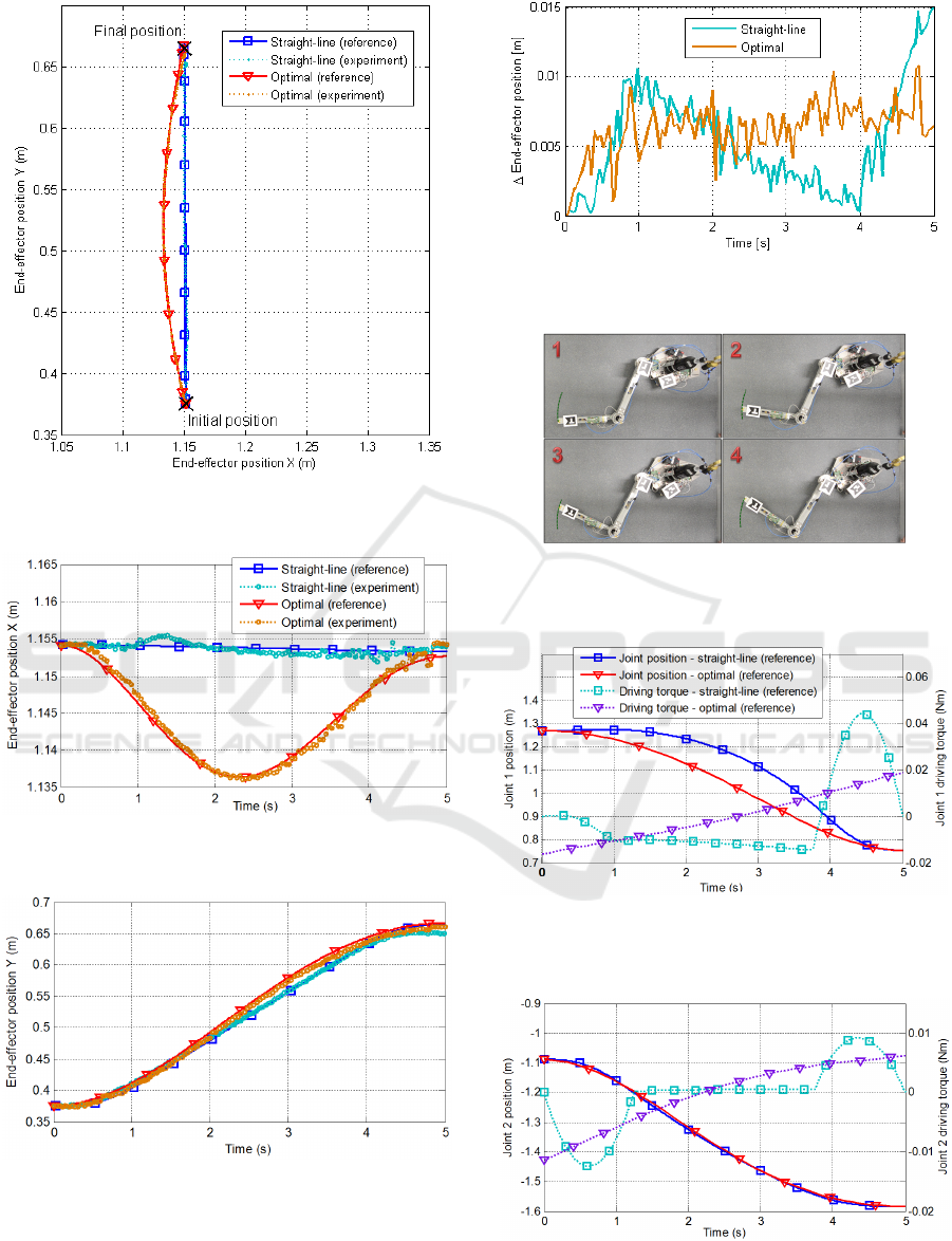
Figure 2: End-effector position on XY plane (straight-line

vs optimal).

Figure 3: X-component of the end-effector position

(straight-line vs optimal).

Figure 4: Y-component of the end-effector position

(straight-line vs optimal).

Figure 5: Difference between the reference end-effector

position and position measured during experiment.

Figure 6: Planar satellite-manipulator system during

realization of the optimal trajectory on the air-bearing

microgravity simulator.

Figure 7: Reference position of manipulator joint 1 and

driving torque applied in this joint (straight-line vs

optimal).

Figure 8: Reference position of manipulator joint 2 and

driving torque applied in this joint (straight-line vs

optimal).

ICINCO 2016 - 13th International Conference on Informatics in Control, Automation and Robotics

5 APPLICATION OF THE

OPTIMIZATION ALGORITHM

FOR A MANIPULATOR WITH

4 DEGREES OF FREEDOM

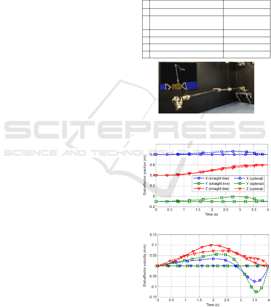
In this section we present the results of trajectory

optimization performed for the WMS1 LEMUR

(Seweryn et al., 2014). A picture of this manipulator

is presented in Fig. 9, while Tab. 2 summarizes its

basic properties. It is a manipulator with 7 degrees

of freedom. However, we perform trajectory

optimization only for the first four joints. The

driving torques required for the positioning of the

end-effector are higher than the driving torques

required for obtaining the desired orientation of the

end-effector. For the manipulator with 7 degrees of

freedom we present results of numerical simulations

only. For the system with a manipulator with 4

degrees of freedom the solution that minimizes

L is

obtained from 40 first order differential equations

and 46 boundary conditions (20 equations

constraining state at

, 20 equations for λ

at t

and

6 equations for ψ).

The initial position of the end-effector (expressed

ine

located at the initial position of the servicing

satellite centre of mass) is r

= t

) = [0.8m -0.1m

0.4m ]

, while the desired final end-effector position

is r

= t

) = [0.8m -0.1m 0.6m]

. The initial and

final velocity of the end-effector is zero. There is no

initial velocity of the servicing satellite. The desired

time of motion is 4

s. As in the case of the planar

system, we use a straight-line trajectory as the initial

guess for the BVP solution and for comparison with

the optimal trajectory. The straight-line trajectory is

divided into a 2

s phase of end-effector acceleration

(in CS

ine

) and a 2s phase of breaking. The position

and velocity of the end-effector for both trajectories

are presented in Fig. 10 and Fig. 11. The positions of

first four manipulator joints are presented in Fig. 12,

while torques applied on these joints are shown in

Fig. 13. In this example the driving torques required

for the realization of both trajectories are far lower

than the maximal available driving torques (15

Nm).

The optimization algorithm allowed 68%

reduction of the cost functional

L (from L

str

= 11.4

opt

= 3.56). Although the final end-effector

position differs from the initial end-effector position

only by Z-component, in Fig. 8 it can be seen that all

components of the end-effector position changed

during the realization of the optimal trajectory (X-

and Y-components return to their initial values at the

end). The boundary condition sets the final end-

effector velocity to zero - this is the main advantage

of the modified algorithm in comparison to its

previous version presented by Seweryn and

Banaszkiewicz (2008). No condition is set on the

final velocities of the manipulator joints. Thus, in

the considered case the final velocities of the

manipulator joints are not equal to zero.

Table 2: Properties of the spatial satellite-manipulator.

Parameter Value

Satellite mass (assumed) 100 kg

Satellite moment of inertia

diag([2.8 6.1 7.4])

kg·m

Number of manip. joints 7

Total length of manipulator 3.1 m

Total mass of manipulator 15.25 kg

Maximal joint driving torque 15 Nm

Figure 9: Prototype of the WMS1 LEMUR robotic arm

and visualization of this manipulator on a servicing

satellite.

Figure 10: End-effector position (straight-line vs optimal).

Figure 11: End-effector velocity (straight-line vs optimal).

Application of Trajectory Optimization Method for a Space Manipulator with Four Degrees of Freedom

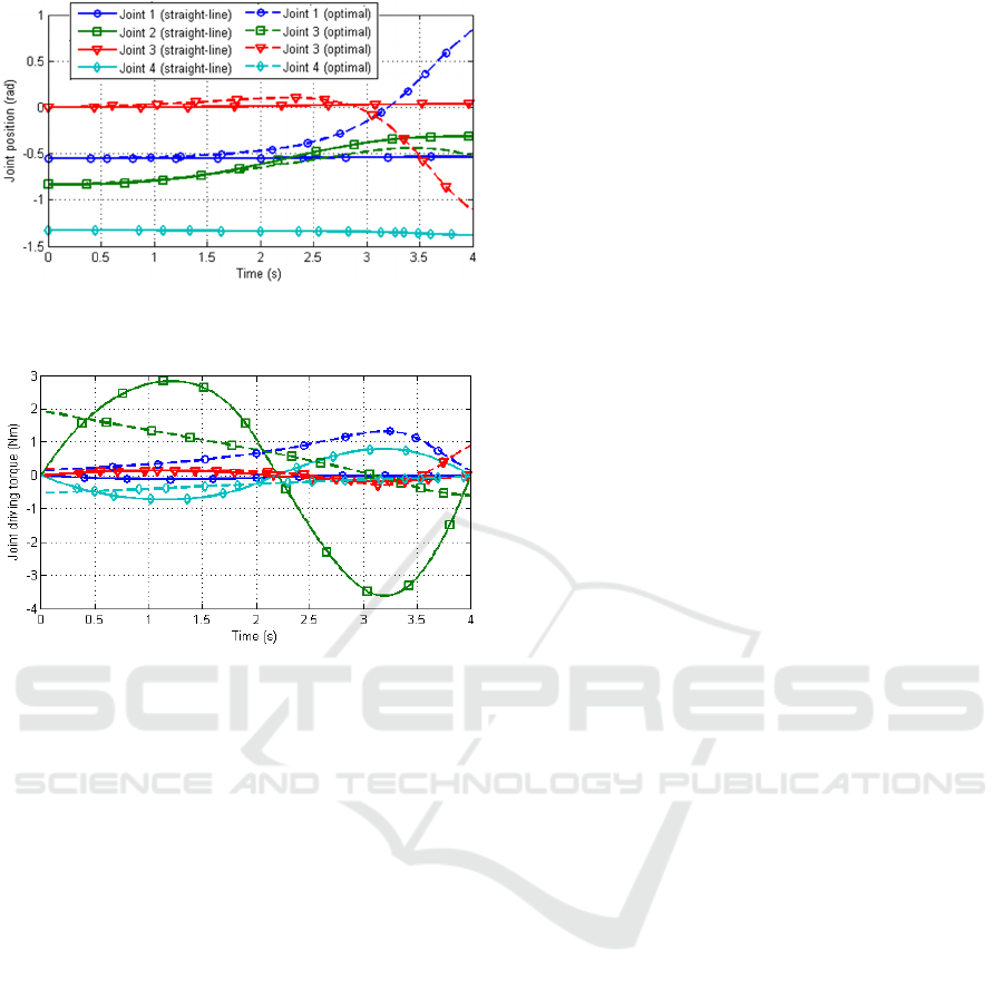
Figure 12: Positions of manipulator joints (straight-line vs

optimal).

Figure 13: Driving torques at manipulator joints (straight-

line vs optimal).

6 DISCUSSION

The use of the trajectory optimization algorithm for

free-floating satellite-manipulator systems was

demonstrated for two cases: (i) a planar system with

a manipulator with 2 degrees of freedom and (ii) a

spatial system with a manipulator with 4 degrees of

freedom (with four joints responsible for obtaining

desired end-effector position). In the first case the

experiments were performed on the planar air-

bearing microgravity simulator. In the second case,

only numerical simulations were performed, but the

mass and geometrical properties of a real prototype

of a space manipulator were used.

As in the approach presented by Seweryn and

Banaszkiewicz (2008) quadratic norm of the control

input has been used as a cost functional that was

minimized. Such approach is simple and common in

automation and robotic. The presented method could

be modified by using a more complex cost

functional that would, e.g., minimize changes in the

satellite orientation. In each case the optimal

trajectory was compared with a straight-line

trajectory and it was proven that the optimization

algorithm allows for substantial reduction of the

power use of the manipulator motors. Moreover, for

the planar case the analysis was performed with 30

trajectories based on randomly selected initial and

final end-effector position and it was found that the

average reduction of the selected cost functional

resulting from the trajectory optimization was

49.4%. In all presented cases the required driving

torques for the manipulator joints were far lower that

the maximal available control torques. However, it is

expected that in the rigidization and detumbling

phases after the orbital capture manoeuvre the

required driving torques will be higher, as the large

mass of the target object will be attached to the end-

effector. In such a case, the presented optimization

method may prove to be very useful.

There are two main weaknesses of the presented

optimization algorithm: (i) it is not guaranteed that

the global minima will be found, and (ii) the

computational cost of the trajectory optimization is

very high. The second issue could be especially

problematic in case of algorithm implementation on

flight hardware. However, the trajectory planning

stage can be performed while the manipulator-

equipped satellite is waiting in a safe point (it might

even be possible to perform such computations on

Earth).

Current work focuses on selecting more practical

cost functional (e.g., to achieve minimization of the

manipulator influence on the satellite) and

performing trajectory optimization after the grasping

of the target object. Precise evaluation of algorithm

computational cost is also currently performed.

7 CONCLUSIONS

Manipulator trajectory planning is important for

planned active debris removal and on-orbit servicing

missions. The successful demonstration of the

trajectory optimization algorithm on the

experimental test set-up (the planar air-bearing

microgravity simulator) was an important step in the

development of this algorithm. The simulations

performed for the spatial manipulator with 4 degrees

of freedom with mass and geometrical properties of

the prototype robotic arm (WMS1 LEMUR) were

also useful for the algorithm validation. Thus, the

results presented in this paper serve not only as an

illustration and example of the optimization

algorithm application, but allow as an assessment of

the possibility of using trajectory optimization

during one of the planned active debris removal and

on-orbit servicing missions.

ICINCO 2016 - 13th International Conference on Informatics in Control, Automation and Robotics

100

ACKNOWLEDGEMENTS

This paper was partially supported by The National

Centre for Research and Development project no.

PBS3/A3/22/2015.

REFERENCES

Aghili, F. (2008) ‘Optimal control for robotic capturing

and passivation of a tumbling satellite with unknown

dynamics’, AIAA Guidance, Navigation, and Control

Conference and Exhibit (AIAA-GNC’2008). Honolulu,

Hawaii, USA, 18-21 August.

Dubowsky, S., Papadopoulos, E. (1993) ‘The kinematics,

dynamics, and control of free-flying and free-floating

space robotic systems’, IEEE Transactions on

Robotics and Automation, 9(5), pp. 531-543.

Flores-Abad, A., et al., (2014a) ‘Optimal Control of Space

Robots for Capturing a Tumbling Object with

Uncertainties’, Journal of Guidance, Control, and

Dynamics, 37(6), pp. 2014-2017.

Flores-Abad, A., et al. (2014b) ‘A review of space

robotics technologies for on-orbit servicing’, Prog.

Aerosp. Sci., 68, pp. 1-26.

Hausmann, G., et al. (2015) ‘E.Deorbit Mission: OHB

Debris Removal Concepts’, 13th Symposium on

Advanced Space Technologies in Robotics and

Automation (ASTRA’2015). Noordwijk, The

Netherlands, 11-13 May.

Junkins, J.L., Schaub, H. (1997) ‘An Instantaneous

Eigenstructure Quasivelocity Formulation for

Nonlinear Multibody’, Dynamics. J. Astronaut. Sci.,

45(3), pp. 279-295.

Kaigom, E. G., Jung, T. J., Rossmann, J. (2011) ‘Optimal

Motion Planning of a Space Robot with Base

Disturbance Minimization’, 11th Symposium on

Advanced Space Technologies in Robotics and

Automation (ASTRA’2011). Noordwijk, The

Netherlands, 12-14 April.

Lindberg, R. E., Longman, R. W., Zedd, M. F. (1993)

‘Kinematic and dynamic properties of an elbow

manipulator mounted on a satellite’, in Xu, Y.,

Kanade, T. (eds.) Space Robotics: Dynamics and

Control. New York: Springer.

Liou, J.-C., Johnson, N.L., Hill, N.M. (2010) ‘Controlling

the growth of future LEO debris populations with

active debris removal’, Acta Astronautica, 66 (5-6),

pp. 648 - 653.

Rybus ,T., Seweryn, K. (2015) ‘Manipulator trajectories

during orbital servicing mission: numerical

simulations and experiments on microgravity

simulator’, 6th European Conference for Aeronautics

and Space Sciences (EUCASS‘2015). Kraków, Poland,

29 June -2 July.

Rybus, T., Seweryn, K., Sąsiadek, J. Z. (2016) ‘Trajectory

Optimization of Space Manipulator with Non-zero

Angular Momentum During Orbital Capture

Maneuver’, AIAA Guidance, Navigation, and Control

Conference (AIAA-GNC’2016). San Diego, California,

USA, 4-8 January.

Rybus, T., et al. (2013) ‘New Planar Air-bearing

Microgravity Simulator for Verification of Space

Robotics Numerical Simulations and Control

Algorithms’, 12th Symposium on Advanced Space

Technologies in Robotics and Automation

(ASTRA’2013). Noordwijk, The Netherlands, 15-17

May.

Seweryn, K., Banaszkiewicz, M. (2008) ‘Optimization of

the Trajectory of a General Free-Flying Manipulator

During the Rendezvous Maneuver’, AIAA Guidance,

Navigation, and Control Conference and Exhibit

(AIAA-GNC’2008). Honolulu, Hawaii, USA, 18-21

August.

Seweryn, K., et al. (2014) ‘The laboratory model of the

manipulator arm (WMS1 LEMUR) dedicated for on-

orbit operation’, 12th International Symposium on

Artificial Intelligence, Robotics and Automation in

Space (i-SAIRAS’2014). Saint-Hubert, Quebec,

Canada, 17-19 June.

Shah, S. V., et al. (2013) ‘Energy optimum reactionless

path planning for capture of tumbling orbiting objects

using a dual-arm robot’, 1st International and 16th

National Conference on Machines and Mechanisms

(iNaCoMM’2013). IIT Roorkee, India, 18-20

December.

Sullivan, B., Akin, D. (2012) ‘Satellite servicing

opportunities in geosynchronous orbit’, AIAA SPACE

2012 Conference and Exposition. Pasadena,

California, USA, 11-13 September.

Umetani, Y., Yoshida, K. (1989) ‘Resolved motion rate

control of space manipulators with generalized

jacobian matrix’, IEEE Transactions on Robotics and

Automation, 5 (3), pp. 303-314.

Application of Trajectory Optimization Method for a Space Manipulator with Four Degrees of Freedom

101