
Hybrid Modeling and Identification of Dynamic Yaw Simulator
Abdelhafid Allad
2
, Lotfi Mederreg
2
, Hocine Imine
1
and Nouara Achour
2
1
The French Institute of Science and Technology for Transport, Development and Networks (IFSTTAR),
Marne-la-Vall
´
ee, Paris, France
2
Department of Intrumentation and Automatic, University of Science and Technology Houari Boumediene, Algiers, Algeria
Keywords:
Dynamic Driving Simulator, Light Vehicle Modeling, Cars Dynamics.
Abstract:
The objective of this work is the study and execution of a dynamic model reproducing the dynamics of a road
vehicle to implement it in a vehicle simulator. To do this we will use a generic approach using Matlab to
model different phenomenons related to the vehicle. In this research, we have taken into account all relevant
parameters in vehicle dynamics, specifying the longitudinal and lateral forces of wheel/ground contact.
For the calculation on an operational dynamic model of the vehicle, we chose the essential compnents to
reduce system complexity while ensuring a degree of realism and effectiveness of modeling, integrating a
status observer by sliding mode to reconstruct or estimate in real-time, the system status.
1 INTRODUCTION
Driving simulators have been becoming little by lit-
tle a suitable tool oriented to improve the knowledge
about the domain of driving research. The investiga-
tions that can be conducted with this type of tool con-
cern both the driver’s behaviour, the design/control of
vehicles, testing assistance systems for driving and
the roadway infrastructures impact. The benefits of
simulation studies are many: lack of any real risk to
users, reproducible situations, time savings and re-
duced testing costs. In addition, their flexibility al-
lows to test situations that do not exist in reality or at
least they rarely and randomly exist.
2 OVERVIEW OF THE DRIVING
SIMULATOR
Motion cueing platforms are widely employed in
driving simulator which became very accessible
through technological progress due to the fact that
computers have become more powerful and less ex-
pensive. Thus, several simulators of various architec-
tures were built with an aim of either human factors
study, or to test new car prototypes and functionali-
ties, or for driver training and education. Most will
agree that inappropriate motion cueing is likely to
induce simulator sickness through multisensory con-
flict. For this reason, the INRETS-MSIS (which be-
came INRETS/LCPC LEPSIS) decided to initiate the
design of a mobile platform aimed primarily at study-
ing the importance of the modalities of yaw render-
ing on virtual vehicle control and on simulator sick-
ness. The aim of the present work is contributing to
improve the performance and the results of this ex-
isting simulator with the creation and insertion of a
new vehicle dynamic model. Dynamic driving sim-
ulator systems allow a driver to interact safely with
a synthetic urban or highway environment via a mo-
tion cueing platform that feeds back the essential in-
ertial components (acceleration and rotation) of the
vehicles movements, in order to immerse the driver
partially or completely. The complexity of dynamic
driving simulators lies in the fact that the system is
composed of interconnected subsystems of different
nature (mechatronics, control laws, computer, etc.) of
which a human subject is an integral part. Dynamic
driving simulators should thus be studied in their en-
tirety, including the human driver.
2.1 Motivation of the Platforms
Architecture Choice
The choices of simulator structure and motion bases
are motivated by the necessity to have a sufficient
perception while driving as well as by financial de-
sign constraints. Thus, the objective of the simulator
project is not to reproduce all of a real vehicles mo-
tions, but only the longitudinal movements (surge),
Allad, A., Mederreg, L., Imine, H. and Achour, N.
Hybrid Modeling and Identification of Dynamic Yaw Simulator.
DOI: 10.5220/0005981605210526
In Proceedings of the 13th International Conference on Informatics in Control, Automation and Robotics (ICINCO 2016) - Volume 1, pages 521-526
ISBN: 978-989-758-198-4
Copyright
c
2016 by SCITEPRESS – Science and Technology Publications, Lda. All rights reserved
521
and yaw. This inertial feedback is to be perceived by
the human user in the intended applications, which
include the study of the effects of yaw cueing on sim-
ulator sickness. Indeed, one of the more nauseat-
ing manoeuvres in a driving simulator is the nego-
tiation of (sharp) curves, especially intersections in
complex environments like agglomerations (S et al.,
2009)(Hichem et al., 2010).
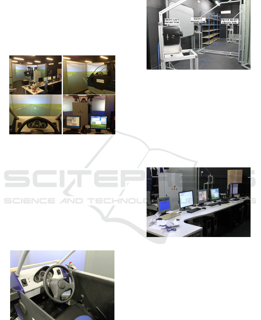
Figure 1: Vehicle simulator.
2.2 Platform Description
Here it is a driving simulator with an acceptable com-
promise between rendering quality, compactness and
cost limitation. The mechatronics components of
the proposed solution are described below (S et al.,
2009)(Hichem et al., 2010):
• The cabin consists of an instrumented mobile part
moving along a guide way mounted on the plat-
form. It is the interface between the driver and
the simulated environment. The cabin is equipped
with acceleration and braking pedals, steering
wheel, gearbox lever and other classical car con-
trol organs. (Figure 2)
Figure 2: Cabin of the vehicle simulator.
• Audio/video generators: the visual output is pro-
vided by a system of five projectors PROJEC-
TIONDESIGN F20 sx + with 1280x1024 resolu-
tion. (Figure 3)
Figure 3: Projector system.
• The acquisition system is composed of an indus-
trial micro controller. This allows the control of
actuators in the desired position, speed or torque
(used for the steering wheel force feedback). A
bidirectional information exchange protocol is de-
fined between this card and the PCs dedicated to
vehicle and traffic models. The communication
is performed through CAN port between the elec-
tronic card and the PC named XPC target: this
one is connected with other PCs by means of Eth-
ernet cables. 5 computers are involved in the data
elaboration and acquisition (Figure 4):
Figure 4: Aquisition system.
3 RELATED WORK
Various studies and researches have been done to edit
a simplified vehicle model by adopting several as-
sumptions with the aim to reduce its complexity in
terms of Degree of Freedom (Dof) and to neglect re-
dundant equations.
3.1 Type of Vehicle Dynamic Model
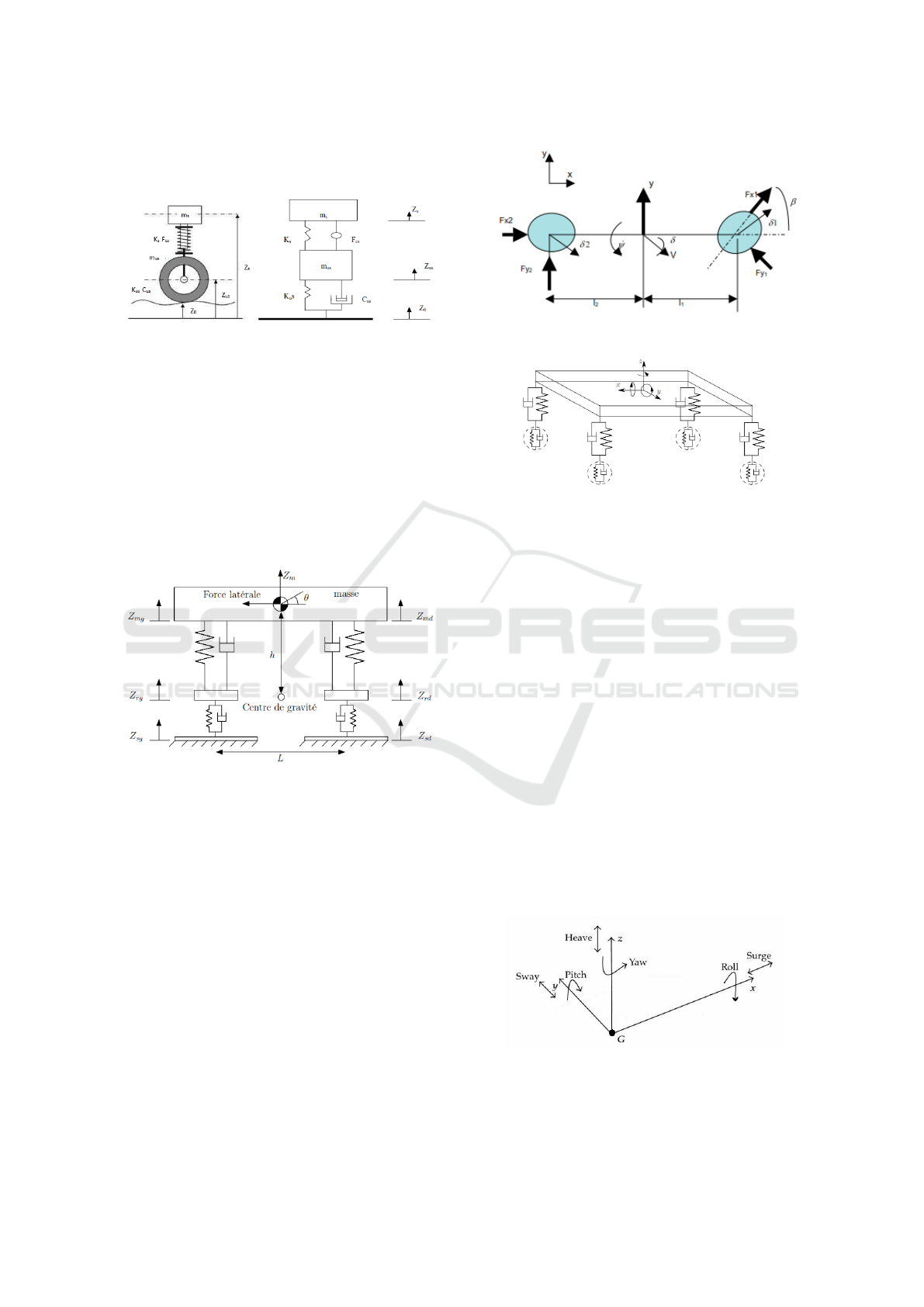
3.1.1 One Wheeled Model (Quarter of Vehicle)
For the study of suspension, the model quarter of ve-
hicle is the simplest one. We find it in previous stydies
ICINCO 2016 - 13th International Conference on Informatics in Control, Automation and Robotics
522
about suspension and pneumatic model with only two
degrees of freedom (NADJI, 2007).
Figure 5: A quarter of vehicle.
3.1.2 Half-vehicle Model
Depending on modelings purpose, in literature it is
possible to find half-vehicle models which, although
far from a complete one, properly accomplish their
tasks (JABALLAH, 2011)(Samuel, 2006).
Lateral Half-vehicle Model. This model represent
a lateral view of the vehicle. It’s used to study roll
mouvements, mathematically il’s a model with four
degrees of freedom.
Figure 6: Lateral Half-Vehicle Model.
Longitudinal Half-vehicle Model (Bicycle Model).
According to simply the model, the 4 wheels system,
supposed a perfect symmetry between right and left
parts, has been reduced to a bicycle model, focusing
the study only to a half car. The forces applied are
simply multiplied by two in order to take into account
the four tires.
3.1.3 Complete Vehicle Modeling
The four wheels model is used for a complet and re-
alistic model of the vehicle dynamics (SLEIMAN,
2010).
4 VEHICLE DYNAMIC MODEL
The proposed dynamic vehicle model is nonlinear.
Figure 7: Longitudinal half-vehicle model.
Figure 8: Complete vehicle modeling.
Moreover, the kinematic elements can greatly influ-
ence the vehicle dynamic behaviour. This is due to
the existing interconnection between different parts of
the vehicle. However, for the sake of simplicity, the
complexity of the model may be reduced depending
on the type of application and the purpose of mod-
elling. Due to the complexity of a complete vehicle
model, the vehicle model is limited to four intercon-
nected subsystems:(VENTURE, 2003)
• The chassis.
• Suspension.
• Wheels and their interaction with the ground.
• The driver controls.
The chassis is treated as an unconstrained body
in the space so it contains six DoFs; since it is con-
sistently integrated with vehicle body, it counts three
DoFs for translation along the longitudinal (Surge),
lateral (Sway) and vertical (Heave) axis and three for
rotations (Roll, Pitch and Yaw); they are all referred
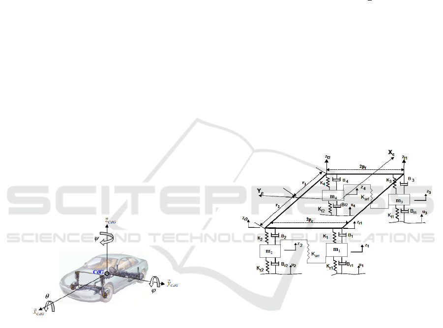
to vehicles Centre Of Gravity (COG) (Figure 9).
Figure 9: Vehicle degrees of freedom.
Its permissible to assume that each tire belonging
to rear axis has two DoFs: one for the rotation and the
Hybrid Modeling and Identification of Dynamic Yaw Simulator
523
other for suspension mechanism translation. Whereas
the front axis is composed by two driving wheels able
to steer, therefore they have one DoF more each (three
DoFs). Finally the entire vehicle system owns 16
DoFs.
4.1 Chassis Dynamic Behaviour
High rigidity of the vehicle chassis can limit its flex-
ibility study and its influence on the suspension sys-
tem and the wheels system. In the present case, the
chassis is considered as rigid. This rigidity helps in
supporting axes with articulations of the elastic type.
Therefore it can be considered as a suspended mass.
The inertial parameters of the body are generally rep-
resented by:
• Its mass m (unsprung mass) and M (total mass of
vehicle) ;
• Position of the centre of gravity G;
• Matrix of inertia J;
The equations of motion of the chassis are ob-
tained by applying the fundamental principles of clas-
sical physics. This leads to three ordinary differential
equations for the translational motion of the centre of
gravity and three ordinary differential equations for
the rotation.
Figure 10: Translational and rotation motion of the centre
of gravity.
4.1.1 Translation Motion
The sum of external forces applied to a solid body
in motion, according to the principle of dynamics, is
equal to its mass m multiplied by its acceleration:
m ˙v
COG
=
∑
F
external f orces
(1)
The equilibrium of these forces along the three axes
leads to the following relation (JABALLAH, 2011):
m
˙
V
x
˙
V
y
˙
V
z
= T
c
r
F
x f 1
+ F
x f 2
+ F
xr1
+ F
xr2
+ F
wx
+ F
gx
F
y f 1
+ F
y f 2
+ F
yr1
+ F
yr2
+ F
wy
+ F
gy
F
z f 1
+ F
z f 2
+ F
zr1
+ F
zr2
+ F
wz
+ F
gz
(2)
Where v = (v
x
, v
y
, v
z
)
T
indicates respectively longitu-
dinal, lateral and vertical velocities.
Forces which contribute to body motion and
which affect it are the following ones:
• Contact Forces: three for each tyre, developed in
the pavement interface (for convention the sub-
scripts f and r indicate respectively front and rear,
whereas 1 and 2 indicate left and right).
• Aerodynamic Forces: F
wx
= −
1
2
C
ax
ρSV
2
x
• Gravity Forces:
F
gx
F
gy
F
gz
= T
s
v
0
0
−mg
The vehicle system is illustrated in the Figure ,
where p
f
and p
r
represent respectively the front and
rear half gauge (the sum of them provides the track
width), whereas r
1
and r
2
represent the distance be-
tween the COG and front and rear axis respectively
(the sum of them provides the wheelbase). m
1
, m
2
,
m
3
, m
4
depict the wheels weight, whereas m is the
sprung mass (of the chassis).
Figure 11: Vehicle With Suspension Model.
The system includes four road inputs u
1
, u
2
, u
3
and u provided by roadway longitudinal profile. The
vertical displacements of the corners Z
r1
, Z
r2
, Z
r3
and
Z
r4
depend on the angles φ and θ and the vertical dis-
placement z of the sprung mass as shown in the fol-
lowing equations (IMINE, 2003):
z
r1
= z − p
r1
sinθ − r
2
sinφ
z
r2
= z − p
r2
sinθ + r
2
sinφ
z
f 1
= z − p
f 1
sinθ + r
1
sinφ
z
f 2
= z + p
f 2
sinθ + r
1
sinφ
(3)
4.1.2 Rotational Motion
In literature it is common to find as the total equilib-
rium of rotational motion around (X
c
, Y
c
, Z
c
) axis the
following expression:
ICINCO 2016 - 13th International Conference on Informatics in Control, Automation and Robotics
524
I
¨
θ
¨
φ
¨
ψ
=
(F
z f 1
− F
z f 2
)P
f
+ (F
zr1
− F
zr2
)P
r
+ (k
arr
+ k
ar f
)θ
−(F
z f 1
+ F
z f 2
)r
1
+ (F
zr1
+ F
zr2
)r
1
(F
y f 1
− F
y f 2
)r
1
− (F
yr1
+ F
yr2
)r
2
+ (F
x f 2
− F
x f 1
)P
f
+ (F
xr2
− F
xr1
)P
r
(4)
where [
¨
θ,
¨
φ,
¨
ψ]represents respectively the accelera-
tions of the roll, the pitch, and the yaw.
The inertia matrix referred to R
c
frame having cross
elements neglected:
I =
I
xx
0 0
0 I
yy
0
0 0 I
zz
(5)
4.2 Global Model
The equations developped before by Newton-euler
laws are synthesized in the state representation below:
˙
ˆ
x
˙x
y
˙y
z
˙z
θ
˙
θ
φ
˙
φ
ψ
˙
ψ
z
1
˙z
1
z
2
˙z
2
z
3
˙z
3
z
4
˙z
4
=
˙
ˆ
x
1
x
2
x
3
x
4
x
5
x
6
x
7
x
8
x
9
x
10
x
11
x
12
x
13
x
14
x
15
x
16
x
17
x
18
x
19
x
20
=
x
2
¨x
x
4
¨y
x
6
¨z
x
8
¨
θ
x
10
¨
φ
x
12
¨
ψ
x
14
¨z
1
x
16
¨z
2
x
18
¨z
3
x
20
¨z
4
(6)
5 SIMULATION AND TEST
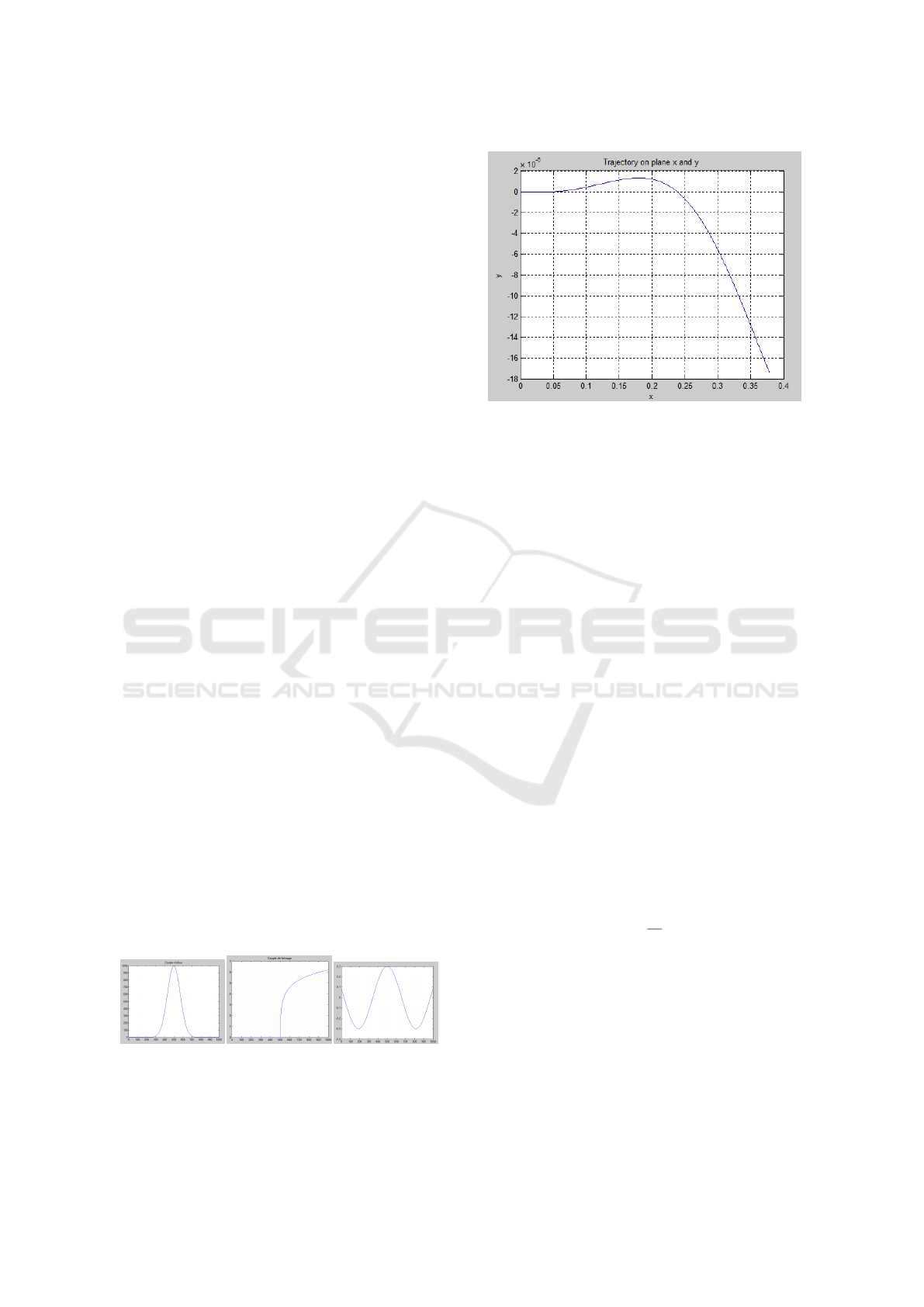
For the tests we had many simulations scenarios, in
the figure below we tested a straight line followed by
two turns:
Figure 12: The simulation conditions: left engine torque,
the brake in the middle and on the right the floor signal.
Figure 13: Result of the trajectories simulated.
We see that the model respect the instructions of
the scenario, but it doesn’t mean that all the vehicle
dynamics are represented, because we neglected some
parameters. We note also, the rotations motions don’t
impacts the trajectory because the undulation of the
road are weak.
5.1 States Estimations
to improve the accuracy of the model, we chose to es-
timate the rotation angles that are the roll, pitch and
yaw. Due to measurements made on an instrumented
car Peugeot 406 provided by IFSTTAR, we compared
these results with what we’ve got in our simulation
model. Using a sliding mode observer we tried to es-
timate the equations that govern the movements of ro-
tations.
The Steps of the Estimate
• the calculation error between the simulated and
measured value
e
θ
= θ
mesur
− θ
calcul
e
φ
= φ
mesur
− φ
calcul
e
ψ
= ψ
mesur
− ψ
calcul
(7)
• Calculation of the sliding surfaces
S = (
∂
∂x
+ γ)e (8)
S
θ
= ˙e
θ
+ γ
θ
e
θ
⇒
˙
S
θ
= ¨e
θ
+ γ
θ
˙e
θ
⇒ −k
θ
sign(S
θ
)
S
φ
= ˙e
φ
+ γ
φ
e
φ
⇒
˙
S
φ
= ¨e
φ
+ γ
φ
˙e
φ
⇒ −k
φ
sign(S
φ
)
S
ψ
= ˙e
ψ
+ γ
ψ
e
ψ
⇒
˙
S
ψ
= ¨e
ψ
+ γ
ψ
˙e
ψ
⇒ −k
ψ
sign(S
ψ
)
(9)
• Study of stability through the theorems lyapunov
We put:
˜w =
˜
θ
˜
φ
˜
ψ
=
θ −
ˆ
θ
φ −
ˆ
φ
ψ −
ˆ
ψ
(10)
Hybrid Modeling and Identification of Dynamic Yaw Simulator
525

We choose the following Lyapunov function:
V (x) =
1
2
S
T
S +
1
2
T
r
( ˜w
T
˜w)
˙
V (x) = S
T
˙
S + T
r
( ˜w
T
˙
˜w)
˙
V (x) = S
T
˙
S + T
r
( ˜w
T
˙
˜w)
(11)
˙
V (x) = (S
θ
S
φ
S
ψ
)
˙
S
θ
˙
S
φ
˙
S
ψ
+ T
r
((
˜
θ
˜
φ
˜
ψ)
˙
˜
θ
˙
˜
φ
˙
˜
ψ
)
(12)
• Equation resolution for obtaining the estimated
variables θ, φ et ψ;
Stability condition:
˙
V (x) ≤ 0 (13)
(S
θ
S
φ
S
ψ
)
˙
S
θ
˙
S
φ
˙
S
ψ
+ T
r
((
˜
θ
˜
φ
˜
ψ)
−
˙
ˆ
θ
−
˙
ˆ
φ
−
˙
ˆ
ψ
) ≤ 0
(14)
The problem posed is to appear
ˆ
θ
ˆ
φ
ˆ
ψ
in the equa-
tions that govern the accelerations, but unfortu-
nately we managed to do it only for 2 variable
from 3. That return us to think about another type
of observation, or downright invites us to recon-
sider our equations.
6 VALIDATION
To determine the reliability of the model we have de-
veloped, we rely on Prosper OKTAL software used
by the world’s leading players in the transport sec-
tor as your: AIRBUS, ENAC, RENAULT, PSA, DGA,
VALEO, SNCF, KEOLIS, RATP, ALSTOM or BOM-
BARDIER. About this tool as an expertise which
refers more and more academic and scientific com-
munity.
7 CONCLUSIONS
This work deals with the topic of modeling and esti-
mating the state of the vehicle subsystems. First, we
looked at different knowledge models and dynamics
of vehicle behavior in the literature. These models
are then used throughout this work based on the prob-
lematic of the study.
The modeling of motor vehicles was developed to
understand their dynamic behavior. Indeed, such a
study has allowed us to understand the complexity of
the various phenomena that interfere in this area.
As regards the aspects of vehicle dynamics; we re-
alized that the most comprehensible way for the study
of vehicle behavior is to split the various dynamics in
parts. In this case, the chassis model, the aerodynamic
forces, gravity, suspension and wheel.
REFERENCES
www.ifsttar.fr.
Boualem, B. (2009). Caracterisation du comportement non
lineaire en dynamique du vehicule. PhD thesis, Uni-
versit de technologie de Belfort Montbeliard, Ecole
Doctoral Sciences pour L’Ingenieur et Microtech-
niques.
Hamadi, N. (2009). Modlisation d’un vehicule en prsence
des forces de contact roues/sol. PhD thesis, Universite
EL-Hadj Lakhdar Batna Algerie.
Hanane, B. (2013). Observateur non lineaire mode glis-
sant. PhD thesis, Universite FERHAT ABBAS Setif
Algerie.
Hichem, A., Salim, H., Lamri, N., Rene J V, B., and
Stephane, E. (2010). From design to experiments of a
2 dof vehicle driving simulator. IEE.
Imine, H. (2003). Observation d’etats d’un vehicule pour
l’estimation du profil dans les traces de roulement.
PhD thesis, Universite de Versailles Saint Quentin en
Yvelines.
Jaballah, B. (2011). Observateur robustes pour le diagnos-
tic et la dynamique des vehicules. PhD thesis, Uni-
versite Paul Cezanne Aix-Marseille III et l’Ecole Na-
tionale d’Ingenieurs de Monastir.
Maakaroun, S. (2011). Modelisation et simulation dy-
namique d’un vehicule urbain innovant en utilisant le
formalisme de la robotique. PhD thesis, Universite de
nantes, Ecole Doctoral de l’ecole des mines de nantes.
Nadji, M. (2007). Adequation De La Dynamique De Ve-
hicule a La Geometrie Des Virages Routiers, Apport
a La Securite Routiere. PhD thesis, Institut National
Des Sciences Appliquees Insa De Lyon.
Ouahi, M. (2011). Observation de systemes e entrees incon-
nues, applications a la dynamique automobile. PhD
thesis, Universite de Limoges Ecole Doctorale ED521
Sciences et Ingenierie pour l’information.
S, E., R, B., P, S., P, P., H, A., S, B., and D, D. (2009). Sim-
ulateur de detection des alterations du comportement
de conduite liees l’attention et la vigilance (vigisim).
Samuel, G.-B. (2006). Etude d’un systeme de controle
pour suspension automobile. PhD thesis, Universite
du Quebec.
Sleiman, H. (2010). Systemes de suspension semi-active a
base de fluide magnetorheologique pour l’automobile.
PhD thesis, Paris Tech, Ecole Nationale Superieure
d’Arts et Metiers.
Venture, G. (2003). Identification des parametres dy-
namiques d’une voiture. PhD thesis, Universite de
nantes, Ecole Doctoral de Nantes.
ICINCO 2016 - 13th International Conference on Informatics in Control, Automation and Robotics
526
