µAUV

- Development of a Minuscule Autonomous Underwater Vehicle

Hendrik Hanff

1,∗

, Korbinian Schmid

2,∗

, Philipp Kloss

and Sven Kroffke

DFKI GmbH − Robotics Innovation Center Bremen, Robert-Hooke Str. 1, 28359 Bremen, Germany

RoboCeption GmbH, Kaﬂerstr. 2, 81241 Munich, Germany

Keywords:

Underwater Robotics, System Design, Miniature Robotics, System Parameter Identiﬁcation, Control of

Underwater Robots, Robot Development.

Abstract:

Small sized robotic systems have operational advantages compared to large systems. They can also operate

in ﬁelds of application where bigger systems would fail. This paper describes the speciﬁcations and the

design of the autonomous underwater vehicle µAUV

. Technical details of the system regarding sensor setup,

motorization and computing power are given. Furthermore, we present details about the system identiﬁcation

process and the implemented controller structure. Possible scopes of the µAUV

are underwater exploration,

inspection tasks, development and evaluation of algorithms, education and competitions.

1 INTRODUCTION

Autonomous underwater vehicles (AUVs) are robotic

systems which do not depend on any input from an

operator. Typical ﬁelds of application include com-

mercial uses e.g. in the oil and gas industry (Albiez

et al., 2015) or the inspection of different underwa-

ter structures, research purposes like the autonomous

investigation of the ice ocean interface, (Dowdeswell

et al., 2008) or even military purposes (Nicholson and

Healey, 2008) like autonomous surveillance tasks.

The development of AUVs is of great interest to all

above mentioned groups. Possible beneﬁts range

from monetary advantages to extended capabilities

due to the extended range of operation.

Dimensions of AUVs range from small, portable

and lightweight to large systems with several meters

length. Large systems offer advantages concerning

payload capacity, range of operation and the ability to

operate when exposed to water currents. In contrast,

small systems offer signiﬁcant advantages during the

launch and recovery process due to their small foot-

print. With their comparably low production and ser-

vice costs, such systems could even be used as dispos-

able sensor units in situations where a recovery is not

possible. Despite these advantages, there only exists a

few small and even less minuscule AUVs. The small

dimensions enable ﬁelds of applications where big-

ger AUVs would fail. One domain might be the ex-

∗

These authors contributed equally to this work.

ploration of underwater cave systems or archaeologi-

cal sites which are too small or too fragile for normal

sized AUVs. Pipeline or wreck inspection could also

be addressed by systems like the presented µAUV

(see Figure 1) or similar systems. Swarms can be real-

ized more easily due to the potentially lower costs per

system. The described system is based on knowledge

from previous projects and the experiences gained

with the µAUV 1 (Fechner et al., 2007) which can

be regarded as the predecessor of the µAUV

The µAUV

, developed at the German Research

Centre for Artiﬁcial Intelligence (DFKI), combines

small dimensions (270x182x156mm

(LxHxW)), a

weight of 1.2kg and a maximum speed of 1.5m/s

with a unique propulsion concept, and high process-

ing power. This paper presents the system design and

development, the identiﬁcation of system parameters

and ﬁrst control approaches.

The main objectives of the µAUV

are the develop-

ment of control and autonomy algorithms. Further-

more the µAUV

represents an easy to use evaluation

platform for swarm algorithms in the underwater area.

2 STATE OF THE ART

In this section, we give an overview of state-of-the-

art AUVs and their unique features which inspired the

development of the µAUV

. A small form factor, an

interesting sensor setup and a streamlined hull are just

Hanff, H., Schmid, K., Kloss, P. and Kroffke, S.

µAUV2 - Development of a Minuscule Autonomous Underwater Vehicle.

DOI: 10.5220/0005982201850196

In Proceedings of the 13th International Conference on Informatics in Control, Automation and Robotics (ICINCO 2016) - Volume 1, pages 185-196

ISBN: 978-989-758-198-4

185

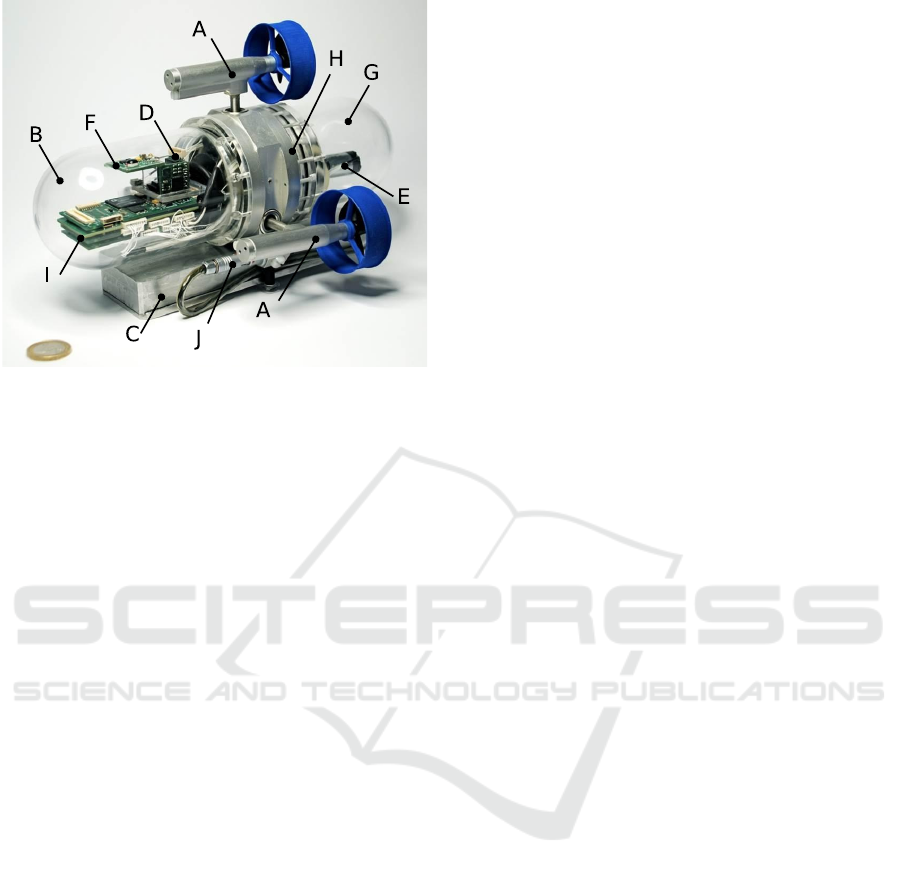
Figure 1: µAUV

- A: DC motor (Maxon motor with in-

tegrated encoder and gear) driven thruster, blue are the 3D

printed protection frames, each of the three thrusters can

be turned ±90

◦

, 3rd thruster cannot be seen in this picture;

B: Front sphere made from acrylic glass; C: battery pack

mounted below the AUV for easy trimming and a low centre

of mass (CM); D: IMU, developed at DFKI GmbH, E: peri-

staltic (buoyancy) pump, a commercialy available product;

F: Optical communication platform; G: Rear sphere made

from acrylic glass; H: Central piece of aluminium which

connects the acrylic spheres and serves as a mounting point

for the three thrusters and the battery pack; I: Printed Circuit

Board (PCB) stack (Microcon1..5) ; J: Connector for the

battery pack. Hidden on the other side of the AUV is the

JTAG connector which permits reprogramming the FPGA

without opening the hull.

some of these features.

The CoCoRo project (Mintchev et al., 2014) has

developed the autonomous underwater vehicles Jeff

and Lily which interact with each other. Each ot the

two AUVs fullﬁlls a different task in a swarm. The 3

degrees of freedom (DOF) Jeff system contains cus-

tom magnetically coupled thrusters and a custom de-

signed rolling diaphragm buoyancy system. A blue-

light sensor system for short-range distance measure-

ment and short-range communication enables the Lily

AUV to fullﬁll swarm operations.

Another example of a small AUV is Monsun

(Meyer et al., 2014). Monsun is a small and inexpen-

sive AUV. Just like CoCoRo, Monsun was designed

to operate in a swarm. Being equipped with an ac-

celerometer, IMU, compass and a camera makes it

ideal for environmental monitoring. Running Linux

and ROS on an ARM based microcontroller provides

a lot of possibilities concerning camera vision. 6

thrusters enable the system to accelerate in all direc-

tions.

Stingray (Barngrover et al., 2011) is a 6 DOF

system and was developed by the San Diego iBotics

group. It consists of a carbon ﬁbre hull which mimics

the shape of the cartilaginous ﬁsh. The streamlined

shape enables the underwater vehicle to maneuver

very energy efﬁcient. In contrast to other small AUVs,

this system makes use of two Voith-Schneider pro-

pellers which make this AUV highly agile. The PC-

104 form factor computer from Kontron comprises an

Intel Core Duo (1.2GHz) with 2Gb of DDR2 RAM

and 100Mbps Ethernet. Being equipped with a cam-

era and a low-cost sonar, the Stingray system is able

to detect underwater objects.

3 SYSTEM DESIGN

Designing a minuscule underwater vehicle poses hard

challenges since commercial of the shelf components

(COTS) do generally not meet the design objectives

mentioned in the introduction. Therefore, hardware

components, electronics as well as mechanics have to

be miniaturized. The system has to provide sufﬁcient

computational power on strictly limited space, ther-

mal and power constraints. Sensors such as cameras

have to be mounted in a way that the acquired data

can be used for navigation as well as inspection tasks.

Electronics has to be protected from water while fast

reprogramming should be possible in a fully assem-

bled state. In the following we describe our system

design considering these aforementioned aspects.

3.1 Mechanics

The main body of the µAUV

consists of three parts:

• 2 hollow acrylic glass domes, one at the front of

the system and one at the back. These two domes

build the hull protecting the inner part of the AUV

from water up to a depth of 2.5 m. Both domes are

transparent to allow optical sensors to monitor the

environment.

• 1 central base frame made of aluminium which

connects the two acrylic domes. This frame also

serves as a carrier for all three thrusters and the

battery pack, see Figure 1, label H.

The AUV has the dimensions 270x182x156mm

(Lx-

HxW).

3.1.1 Propulsion

3 thrusters are responsible for moving the µAUV

all directions. The top thrusters can be turned in-

dependently ±90

◦

. The two side thrusters can be

synchronously turned ±90

◦

. All thrusters are pro-

pelled by Maxon RE 10 DC motors in a 6V/1.5W

ICINCO 2016 - 13th International Conference on Informatics in Control, Automation and Robotics

186

conﬁguration. In combination with the epicyclic 16:1

gear Maxon GP10a1 and the Maxon quadrature en-

coder MR S 16 they actuate the µAUV

. All three

thrusters can be rotated by Krick micro pile gear mo-

tors whose current angle of rotation is measured with

potentiometers (Schmid, 2008). The conﬁguration

and the high ﬂexibility of the thrusters make the AUV

highly agile compared to miniaturized AUVs in its

class (see Section 2))

3.1.2 Buoyancy Tank

Like the CoCoRo system (see Section 2 ) the µAUV

also contains a buoyancy tank. This buoyancy or bal-

last water tank enables the µAUV

to ﬂoat energy ef-

ﬁciently at a certain depth in the water column. The

tank can be ﬁlled and emptied with a peristaltic pump.

The ballast water tank itself is a simple convoluted

rubber gaiter. To prevent an overﬁlled water tank,

the status (full/not full) of the water tank is measured

with an ordinary mini push-button switch. The ﬁll

level is determined by measuring the time the pump

is switched on while the throughput of the peristaltic

pump is known.

3.2 Electronics

The main electronics were designed with modularity

and miniaturization in mind. It consists of 5 stackable

PCBs (Printed Circuit Boards) named Microcon 1, 2,

3, 4 and 5 respectively. All PCBs have the same form

factor and are thus stackable . This concept enables

an easy extension by further electronic components if

needed. Microcon1 is responsible for driving the mo-

tors, generating the system voltage and for determin-

ing the motor current. The second board contains the

communication hardware: 4 UARTs for serial com-

munication, 8 GPIOs and in addition 3 eight channel

ADCs. Microcon3 is the processing board. It em-

beds a Xilinx Virtex 4 FPGA (XC4VLX25) with an

8Mbit conﬁguration Flash and 512k x 8 bit low volt-

age SRAM. Microcon4 houses a Blackﬁn DSP, static

memory and ﬂash memory. Microcon5 houses a cam-

era (see Section 3.2.1) and the corresponding elec-

tronics. All PCBs offer a small form factor of only

35x80mm.

The µAUV

contains several complementary sen-

sors to control the thrusters and to navigate au-

tonomously under water.

3.2.1 Camera

For environmental perception the µAUV

is equipped

with two ON Semiconductor MT9V022 digital cam-

eras, one pointing downward and one pointing ahead.

With a wide VGA resolution (752Hx480V), global

shutter, a frame rate of 60fps and optional 8 bit serial

(LVDS) or 10 bit parallel video data output, the cam-

era is ideal for machine vision tasks. Being connected

to an FPGA, the machine vision algorithms can be

accelerated with minimum power consumption com-

pared to CPU or GPU computation.

3.2.2 IMU

To measure the attitude of the vehicle, an Inertial

Measurement Unit (IMU) was developed. The µIMU

has a size of 20x20x20mm and consists of 1 gyro-

scope per axis, a three-axis acceleration sensor and a

three-axis magnetometer . An on-board controller ﬁl-

ters and fuses the sensor values with a Kalman ﬁlter

(Kalman, 1960) and calculates the quaternions to de-

termine the actual attitude of the system. The data is

sent to the central processing unit via UART.

3.2.3 Differential Pressure Sensor

The differential pressure sensor Freescale

MPX5100DP is used to determine the depth of

the vehicle. With a sensitivity of 45mV/kPa and

a range from 0 to 100kPa the sensor will deliver

4.5mV/cm. The 12 bit ADC which transforms the

analog output into the digital domain has a resolution

of 240µV /bit leading to a depth resolution of 1.8mm

per bit.

3.2.4 Thruster Attitude Sensor

The current inclination of the thrusters can be mea-

sured by potentiometers (Piher N15TV) which are

mounted on the turning axis. Linear potentiometers

change their voltage division ratio proportional to the

angle of rotation of the shaft of the potentiometer. Us-

ing an analog to digital converter (ADC) the output

voltage of the potentiometer can be converted into the

digital domain. Thus the determined inclination of the

thrusters is used for control.

3.2.5 Thruster and Pump Speed Sensors

The speed of the thruster and pump motors is mea-

sured with quadrature encoders.

As already mentioned in Section 3.1.1, the used

quadrature encoder is a Maxon MR S 16. The sensor

delivers 16 counts per turn and in combination with

the used 16:1 Maxon gear, 256 counts are produced

for one 360

◦

shaft revolution. Maximum electrical

and mechanical speeds are 30000rpm.

µAUV2 - Development of a Minuscule Autonomous Underwater Vehicle

187

3.2.6 Communication Module

Underwater wireless communication is still an area of

research. Depending on the transmission power, high

speed communication methods like WLAN or Blue-

tooth usually last less then 10cm. This is because the

attenuation of frequencies in the range of radio waves

in water is very high compared to the attenuation in

air due to the dipol nature of the water molecules

(Bryant, 2002) . Long range communication channels

like Long Baseline Modems (LBLs) are too bulky for

a miniaturized AUV and due to their low frequency

range acoustic methods do not have the capability to

transmit a huge amount of data in an appropriate time.

In contrast, optical communication methods pro-

vide a throughput which is high for certain wave-

lengths. A very low attenuation (2 · 10

−2

/m) appears

for a wavelength of 480nm. Thus the µAUV

equipped with an optical communication module that

was developed at the DFKI. This means of communi-

cation was also chosen because the range that is cov-

ered by optical underwater communication modules

easily covers the dimensions of the basin that is avail-

able for tests at the DFKI GmbH. Data is sent with

a green (530nm) LED. An OTS IrDa (infrared data)

transceiver (Maxim Integrated MAX3120) physical

layer is used for controlling the LEDs. The complete

OptCom module is UART compatible and ﬁts on one

of the PCBs mentioned in section 3.2. The datarate

achieved is 19.2kbps with a range of approximately

2.5m.

4 SYSTEM PARAMETER

IDENTIFICATION

The system model introduced by (Fossen, 2002)

builds the basis for the controller. The identiﬁcation

process of the corresponding model parameters as de-

scribed in (Indiveri, 1998) and (Ridao et al., 2001) is

described in this Section.

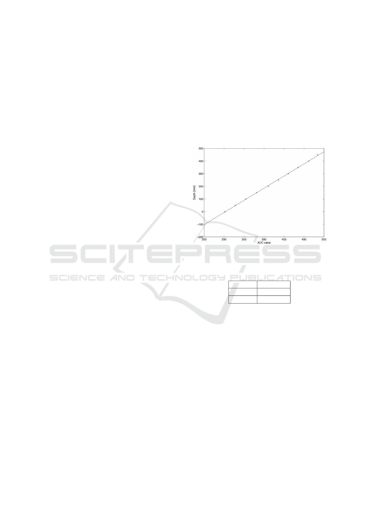
4.1 Pressure Sensor

The diving depth of an underwater vehicle can be cal-

culated by Equation 1, where p is the hydrostatic pres-

sure [Pa], h is the depth in meter, ρ is the density of

water [kg/m

] and g is the gravitational acceleration

(9.81 m/s

p = hρg (1)

The pressure sensor provides information about

the current pressure surrounding the AUV. Equation

2 is used to convert sensor output data into depth

information,

d(V ) = C

V +C

(2)

where d(V) is the depth, V is the output voltage of

the sensor, C

is a constant factor and C

is an offset.

For identifying the constants C

and C

, the µAUV

is manually submerged to a depth of 50cm which is

the maximum depth of the available pool. The system

was then ascended in steps of 5cm.

We used linear regression to identify the constants

(see Table 1 and Figure 2).

Figure 2: The sampled pressure sensor output data with lin-

ear resgression (Schmid, 2008).

Table 1: Results of the system identiﬁcation of the pressure

sensor.

1.920m/V

-486.4mm

static 0.993

4.2 Thrusters

The following one-state thruster model was proposed

by (Yoerger and Slotine, 1991)

τ = C

n|n| (3)

˙n = βT − αn|n| (4)

where τ is the output force, C

, α and β are sys-

tem constants, n is the propeller revolution rate and

T is the input torque. Due to the usage of small

and lightweight propellers, the time constant of the

thrusters is assumed to be very small compared to the

time constant of the system. Therefore the thruster

dynamics can be neglected. C

varies depending on

the sign of the revolution rate (forward/backward) and

is thus denoted as C

and C

−

. The experimental set-

up to identify the thruster force parameters is depicted

in Figure 3. The µAUV

is in the middle of the pool

while it is attached to an aluminium rod. Outside of

ICINCO 2016 - 13th International Conference on Informatics in Control, Automation and Robotics

188

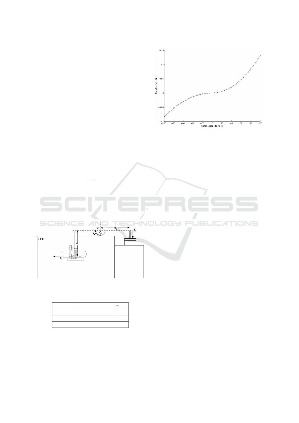
the pool is a scale on which the µAUV

generates a

force when the thrusters are turned on. This is due

to a mechanical connection between the AUV and the

scale via a lever arm.

The speed of the side thrusters is increased syn-

chronously from −100% to +100% in steps of 5%

while the related weight on the scale is saved. The

torque that is generated in point O by the force of the

two side thrusters can be calculated using Equation 5.

= 2 f

(5)

is the torque in point O, f

is the thrust of one

thruster and d

is the perpendicular distance of the

thrusters from O. On the scale a force f

is induced by

the torque τ

which can be determined by equation 6

= m

(6)

where m

is the measured weight on the scale, g is

the gravitational constant and d

is the length of the

arm between O and the point of contact on the scale.

Using Equations 5 and 6, the resulting thruster force

can be calculated as

g (7)

With f

= τ from Equation 3 we ﬁnd

g = C

n|n| (8)

Linear regression on the measured (m

,n) tuples (see

Figure 4) reveals the parameter C

Scale

Figure 3: Thruster force identiﬁcation experiment set-up

(Schmid, 2008).

Table 2: Results of the experiments with the thrusters.

13.2 · 10

−06

Nm(

)

−

−8.32 · 10

−06

Nm(

)

static 0.9990

2−

static 0.9989

4.3 Damping Coefﬁcient

The motion of a moving, submerged object is damped

by friction generated by the surrounding liquid parti-

cles (Fossen, 2002). The following assumptions are

Figure 4: Thruster force over revolution rate including lin-

ear regression(Schmid, 2008)).

made to reduce the complexity such that the damping

coefﬁcients can be determined experimentally.

1. Only steady state movements without linear ac-

celerations are considered

2. Only linear movements are considered

3. The AUV is stable with zero buoyancy and no roll

and pitch are assumed

4. In contrast to the deﬁnition by (Fossen, 2002)

where D is a complex function depending on ν,

we use the approximation of (Leonessa, 2008)

in Equation 9 for linear and quadratic damping

(Christensen et al., 2009).

ν = [u v w p q r]

represents the position in

a body ﬁxed system {B

xyz

} in all 6 degrees of free-

dom.

D = − diag(X

)

D(ν) = − diag(X

u|u|

|u|,Y

v|v|

|v|,Z

w|w|

|w|,

p|p|

|p|,M

q|q|

|q|,N

r|r|

|r|)

(9)

D(ν)ν = τ



















0 0 0 0 0

0 Y

0 0 0 0

0 0 Z

0 0 0

0 0 0 K

0 0

0 0 0 0 M

0 0 0 0 0 N

























u|u|

|u| 0 0 0 0 0

0 Y

v|v|

|v| 0 0 0 0

0 0 Z

w|w|

|w| 0 0 0

0 0 0 K

p|p|

|p| 0 0

0 0 0 0 M

q|q|

|q| 0

0 0 0 0 0 N

r|r|

|r|



















(10)

are linear and

u|u|

|u|,Y

v|v|

|v|,Z

w|w|

|w|,K

p|p|

|p|,M

q|q|

|q|,N

r|r|

|r|

µAUV2 - Development of a Minuscule Autonomous Underwater Vehicle

189

are quadratic damping factors. Under the mentioned

assumptions the six degrees of freedom can be

separated such that each degree of freedom is an

equation of the form

max

+ D

ν|ν|

max

|ν

max

| = τ

(11)

with v

max

as the constant maximum velocity at an

input force/torque of τ. Because only heave and

yaw will be controlled actively in a closed loop

conﬁguration, the only parameters that need to be

identiﬁed to determine suitable controller parameters

are Z

, Z

w|w|

, N

and N

r|r|

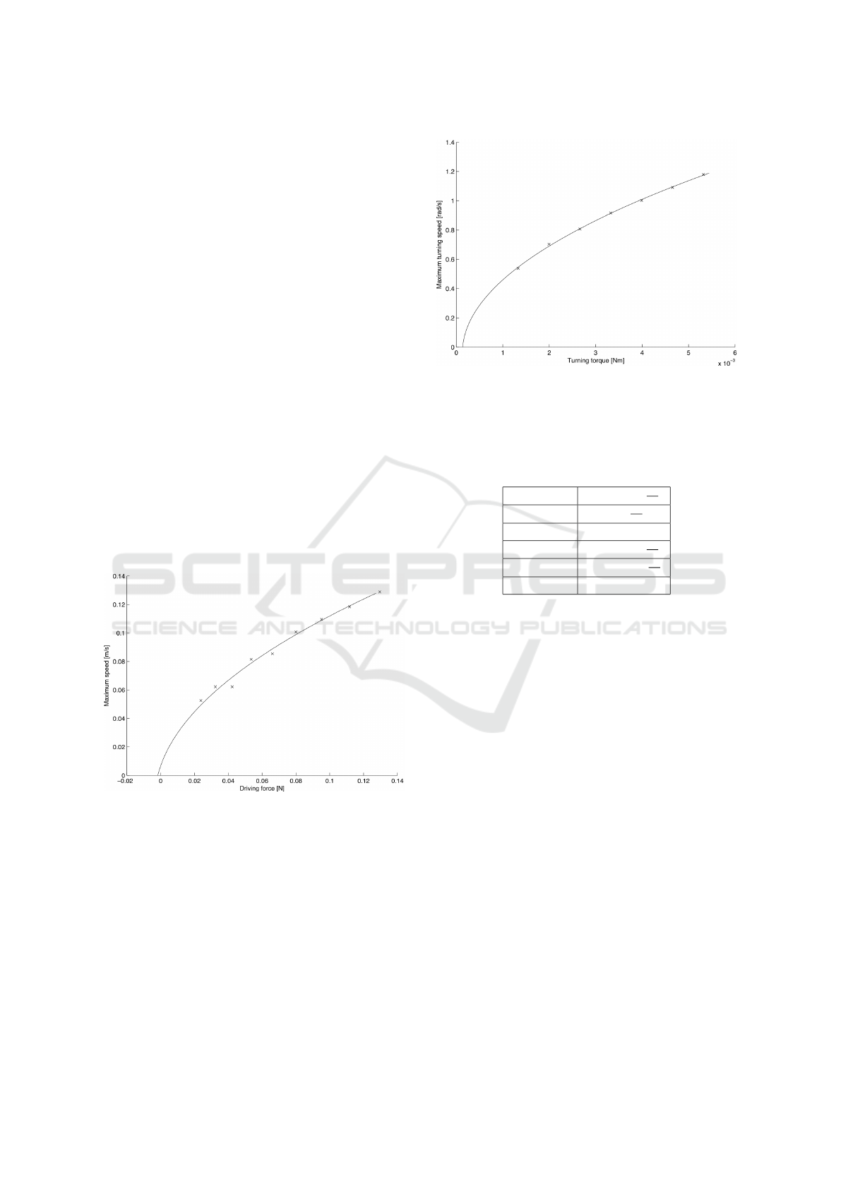
The experimental setup for the identiﬁcation of

the heave parameters was as follows: The µAUV

was submerged to the bottom of the pool. Then it

emerged with a constant thruster force which was

varied in subsequent experiment runs. The diving

speed is determined by the derivation of the pressure

sensor data. The (w

max

,Z) tuples are the sampling

data for a linear regression on Equation 11. The

heave position was measured with varying values for

Z = [0.0238 0.0324 0.0423 0.0535

0.0661 0.08 0.0952 0.1117 0.1295]N. Figure

5 shows the result of the regression and the maximum

reachable heave speed over the applied force. The

results can be seen in Table 3.

Figure 5: Maximum heave speed over driving force

((Schmid, 2008)).

To identify the yaw damping, the experimental

setup starts with positioning the µAUV

in the mid-

dle of the pool. Then a deﬁned and constant torque

is applied to both side thrusters. The torque is varied

with each consecutive run of the experiment. The yaw

turning speed is logged from the IMU. Different yaw

speeds were measured for the corresponding torques

τ = [0.0013 0.0020 0.0027 0.0033 0.0040

0.0047 0.0053]Nm.

Figure 6 shows the resulting regression function

and the measured maximum yaw speed samples.

Figure 6: Maximum yaw speed over driving force with re-

gression function ((Schmid, 2008)).

The results of the experiments are summarized in

Table 3.

Table 3: Results of the damping experiments.

204 · 10

−3

w|w

|w| 6.28

static 0.9902

251 · 10

−6

r|r|

|r| 3.54 · 10

−3

static 0.9990

4.4 Additive Mass

In this section, the added mass of the vehicle is esti-

mated. The added mass is an extra virtual mass term,

since an accelerating or decelerating body must move

some volume of the surrounding ﬂuid as it moves

through it (Fossen, 2002).

If we assume that:

1. The vehicle is accelerating such that ˙v 6= 0

2. The movement of the AUV is linear along one

axis

3. Buoyancy, roll and pitch are zero

the system equation from (Fossen, 2002) can be sim-

pliﬁed to

τ − D(ν)ν = (M

+ M

)

ν (12)

with M

+ M

= M (M

= mass of the rigid body

and M

=additive mass) being the only parameter, be-

cause the damping coefﬁcients were already identiﬁed

in Section 4.3. τ are the forces/torques in a body ﬁxed

system {B

xyz

}. The degrees of freedom in Equation

12 are assumed to be separable resulting in Equation

τ − D(ν)ν − D

ν|ν|

ν|ν| = M

ν (13)

ICINCO 2016 - 13th International Conference on Informatics in Control, Automation and Robotics

190

The total effective mass parameter M can be identi-

ﬁed with a linear regression on Equation 13 and the

data tuples (τ − D(ν)ν − D

ν|ν|

ν|ν|,

ν). Measurements

show that the above mentioned condition

ν 6= 0 is

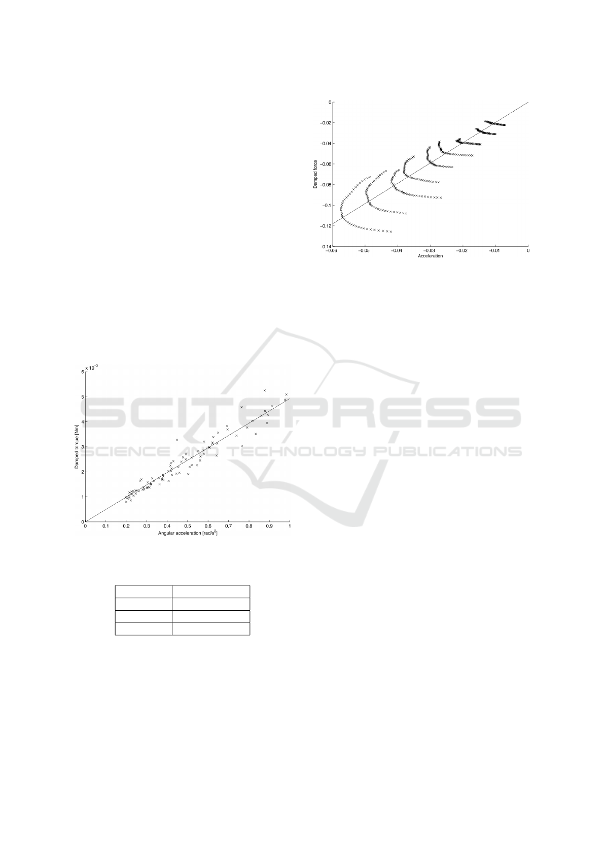
true between t = 1.5s and t = 3s. Figure 7 shows the

ﬁtted regression result with the regression input data

tuples. Table 4 lists the regression results.

Identifying the effective mass for heave is more

critical than for yaw because the current depth is the

only measurable system state and Equation 13 needs

the ﬁrst and second derivative of the depth. The IMU

acceleration sensors do not permit to detect small

changes in acceleration due to a low resolution and

noisy signals of the sensors. Therefore, the second

derivative needs to be determined numerically which

is badly conditioned as high frequency noise is am-

pliﬁed. Measurements showed that the acceleration

phase is between t = 2.5s and t = 3.5s. A regression

line through the data tuples can be seen in Figure 8.

The coefﬁcient of determination R

is very bad with a

value of 0.80.

Figure 7: Damped yaw torque over acceleration ((Schmid,

2008)).

Table 4: Additive mass parameters.

4.9 · 10

−3

kg · m

static 0.9990

1.96kg

static 0.80

5 SYSTEM CONTROL

The system model and the identiﬁed parameters are

the basis for the layout of the controller system. This

section will begin with deﬁning the system properties.

Then the controller structure will be explained in de-

Figure 8: Damped heave force over acceleration ((Schmid,

2008)).

tail providing both information about the simulation

and information about the implemented controller.

5.1 µAUV

System Properties

Tests showed that the µAUV

is stable concerning roll

and pitch as long as the thruster controllers only gen-

erate low frequency thruster angle changes. Thus both

roll and pitch are controlled passively. In the follow-

ing the angles α and β are related to the orientataion

of the top- and side thrusters respectively. The follow-

ing modes were deﬁned to control the µAUV

1. Diving mode, α = 0,β = −π/2. Top thruster

turned off. Used for pure heave control

2. Buoyancy mode: diving with pump control

3. Turning mode: α = 0,β = 0 Top thruster turned

off. Used for pure yaw control

4. Drift mode: α = π/2,β = 0. Top thruster turned

off. Used for pure yaw control

5. Auto mode: α = 0,β ∈ [−π/4;π/4]. Used for

concurrent heave, yaw and surge control

5.2 Controller Structure

We ﬁrst designed a simulation to test the AUV con-

trollers: Figure 9 shows the block diagram of the sim-

ulated control system.

Inputs are in absolute values for heave and yaw in

xyz

}, desired thruster forces for surge and sway in

xyq

} and the mode of the controller. The block la-

beled CTRL1 is the implementation of the controller.

It will be described in detail in this paragraph. Con-

troller output thrust is limited by the saturation block

to the maximum thrust of the used thrusters. A mov-

ing average lowpass ﬁlter is used to suppress fast

thruster movements related to the fast changes in the

µAUV2 - Development of a Minuscule Autonomous Underwater Vehicle

191

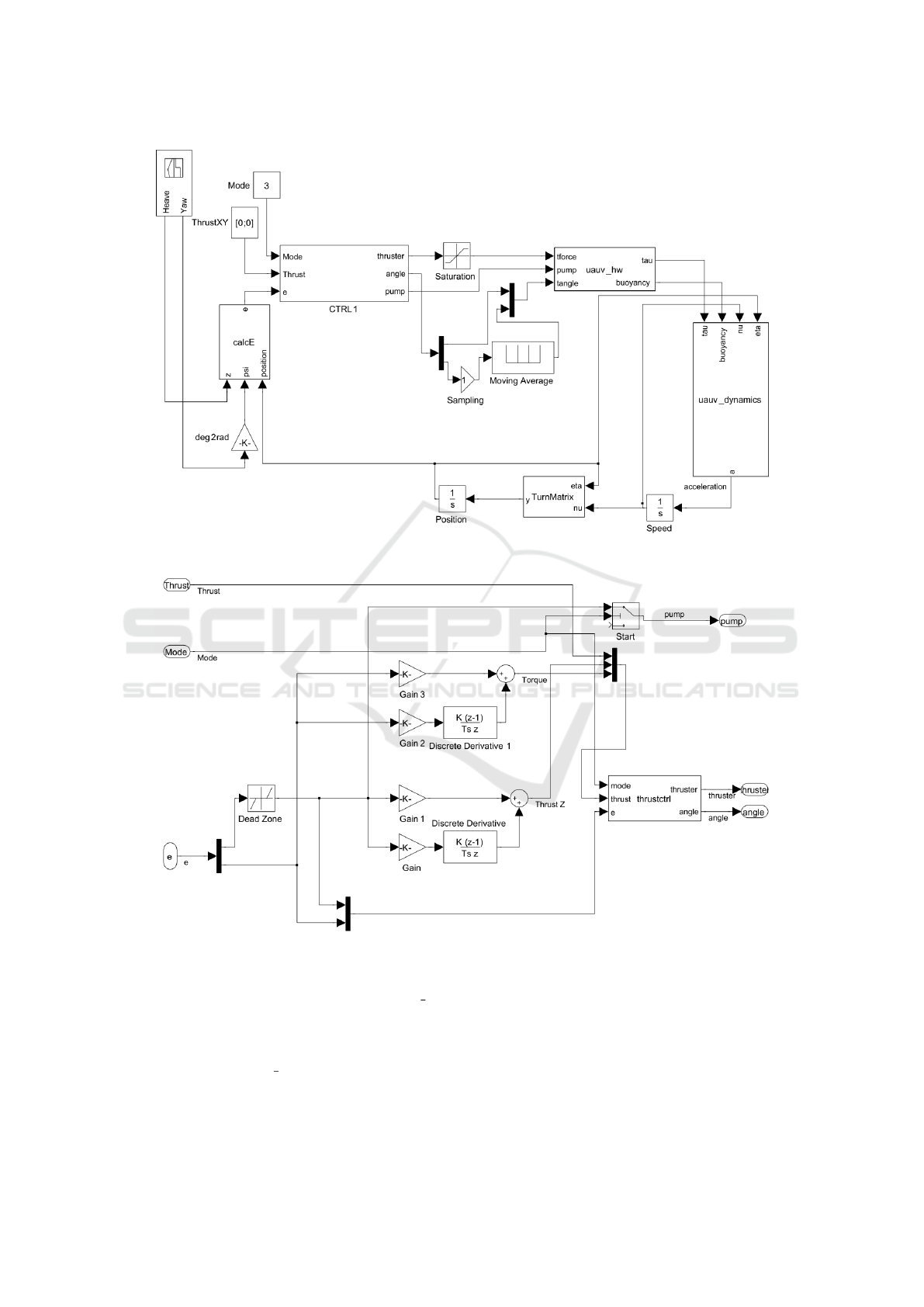
Figure 9: Block diagram of the complete control system ((Schmid, 2008)). Inputs are on the left and outputs are on the right.

Figure 10: Detailed CTRL1 block diagram (Schmid, 2008).

output of the related controller because these might

destabilize the µAUV

. The block labeled uauv hw

transforms thruster force to applied force in {B

xyq

In addition it is responsible for controlling the buoy-

ancy state. The system equation from (Fossen, 2002)

is modeled in block uauv dynamics to determine the

system acceleration against the current system states.

To get the system speed the acceleration state is inte-

grated over time. This value is fed back to the system

dynamic block. A transformation matrix is used to

transform the system speed from {B

xyq

} to {W

xyq

This speed vector is integrated to determine the posi-

tion of the system. The resulting value is fed back to

both the turning matrix and the AUV dynamics block.

To calculate the heave and yaw controller error the

position is used. Please keep in mind that the system

ICINCO 2016 - 13th International Conference on Informatics in Control, Automation and Robotics

192

only implements the actively controlled DOF.

Figure 10 shows a detailed block diagram of the

implemented controller block CTRL1. The error in-

puts for heave and yaw are used as inputs for two PD

controllers. A heuristic method was used to estimate

the values for P- and D in simulation. Fine tuning of

the parameters was done in the water basin. Depend-

ing on the controller mode, the PD controller outputs

as well as the rest of the CTRL1 block inputs are used

for thrust and angle calculation. In buoyancy mode,

a bang-bang controller was used for the pump with a

dead zone on the heave error.

5.3 RESULTS

A minuscule AUV named µAUV

has been techni-

cally described in this paper. The system was suc-

cessfully tested in waterbasins at the DFKI GmbH

in Bremen, Germany. System parameters have been

identiﬁed experimentally. They have been the basis

for the controller design. This section presents the

main simulation and experimental results.

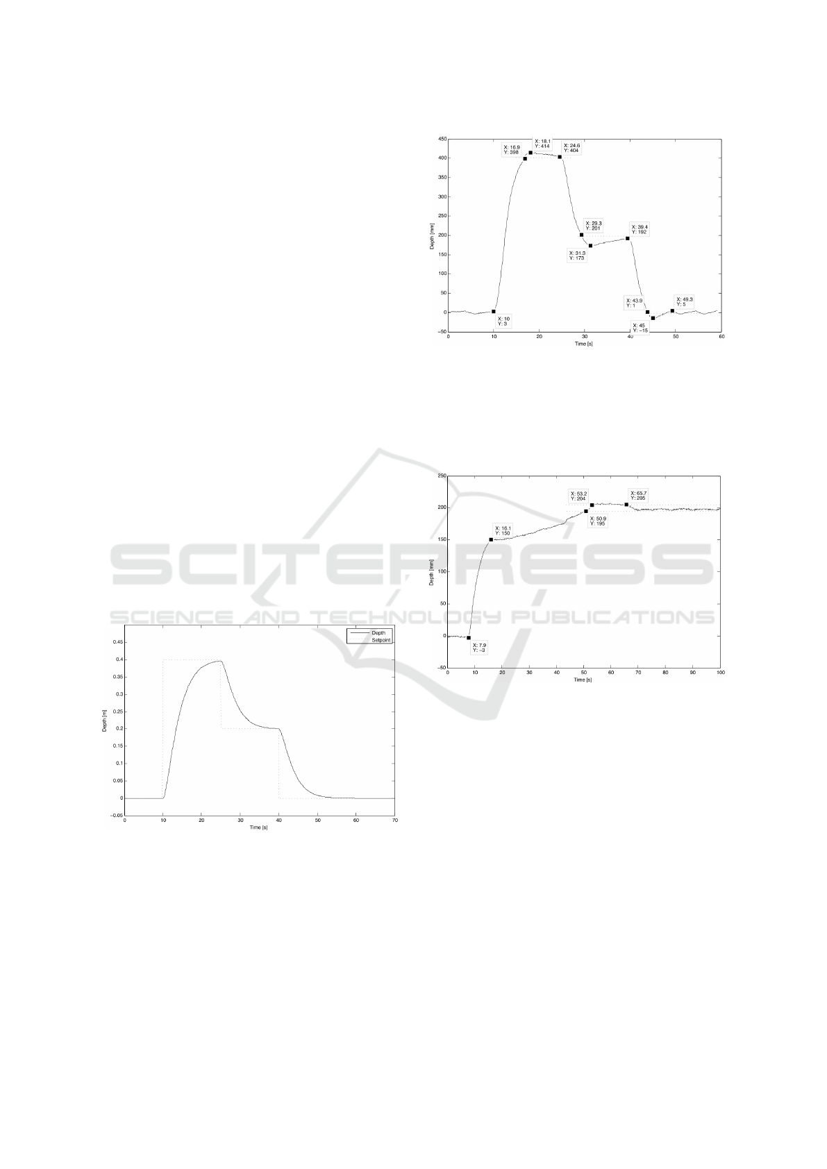
5.4 Diving Control

To analyse the performance of the diving controller, a

diving trajectory was deﬁned. Starting at the surface

of the water, a new depth value of 0.4m is set after

t=10s. 15s later the value is changed to 0.2m. At

t=40s the depth is set to 0m.

Figure 11: Diving controller in simulation (Schmid, 2008).

The trajectory was used for simulation (Figure 12)

and real runs (Figure 12). In simulation the system

shows no overshoot for ω

= 0.6 as ζ

= 1. The sys-

tem successfully reaches the setpoints after 15s. In

reality the system reacts much faster. Setpoints are

reached after 7s. The determined error of 8mm is very

low.

Figure 12: Diving controller on a real run (Schmid, 2008).

5.5 Buoyancy Control

A buoyancy calibration run before each system start

is crucial because the depth controller is designed for

zero buoyancy.

Figure 13: Buoyancy compensation run (Schmid, 2008).

The calibration can be seen in Figure 13. It starts

by setting the depth to 0.2m while the µAUV

has a

positive buoyancy. A depth of 0.15m is reached af-

ter 16s. The PD controller has a steady state error of

0.05m. After 51s the pump has reduced buoyancy so

much that the dead zone is reached. 2s later the dead

zone is left again because a negative buoyancy was

reached. The system reacts by increasing the buoy-

ancy such that the system re-enters the dead zone.

Now a zero buoyancy state is reached.

The control effort was chosen low (ω

= 0.4) on

purpose to avoid large overshoots which could even

lead to oscillations. Once the dead zone is reached

the system stays in the dead zone of 8mm for at least

30s.

µAUV2 - Development of a Minuscule Autonomous Underwater Vehicle

193

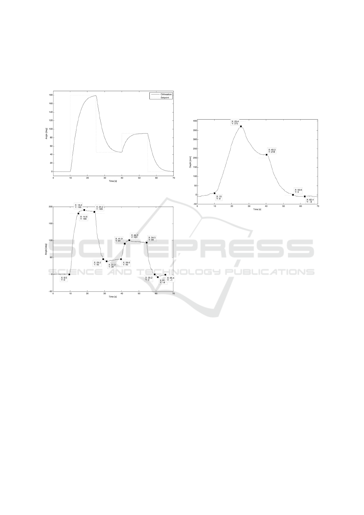
5.6 Turning Control

Again a trajectory was deﬁned to evaluate the turning

control mode.

Figure 14: Simulation results of the turn controller (Schmid,

2008).

Figure 15: Turning control with ω

= 0.6 and increased

DΨ

= 0.016 (Schmid, 2008).

The simulation can be seen in ﬁgure 14. It starts at

an orientation of 0

◦

. After 10s, the set point becomes

180

◦

, 15s later it is set to 45

◦

for 15s to jump to 90

◦

at a time of 40s. At 55s the orientation is reset to

◦

. To reduce overshoots the K

Dψ

part was increased.

The maximum overshoot is 10

◦

which corresponds to

2.8% of the total angle range of 360

◦

. The controller

reaches a maximum average turning speed of 34

◦

which is about 60% of the maximum possible turning

speed of the µAUV

(see Figure 15).

5.7 Auto Mode Control

To compare both the diving and turning controllers

with the auto mode controller the same trajectories

mentioned in the corresponding sections were created

for the auto mode controller. Surge and sway mo-

tion should be suppressed by the controller. The side

thruster angle does not permit high frequency move-

ments (except for the steps at a set point change which

is acceptable). Surge and sway stayed at zero for

the whole simulation time. The top thruster could

perfectly compensate the surge force of the two side

thrusters. In reality, the auto heave controller is a lot

slower than the diving controller, see Figure 16.

Figure 16: Performance of the auto mode controller, heave

(Schmid, 2008).

The maximum average speed of 0.0024m/s is less

than the half of the depth control performance. The

effect can be explained with the thruster saturation.

The total surge force that is produced by the side

thrusters is limited to the maximum thrust level that

the top thruster can produce to compensate the surge

motion and stay at the same place. This also reduces

the thrust that is used for diving. It can also be seen

that overshoots mentioned before disappeared and a

steady state error of a maximum of 0.018m could be

reached. In relation to the total pool depth of 0.6m,

the error is still acceptable.

The maximum average turning speed is only

slightly reduced to 28

◦

/s (compared to 34

◦

/s in turn-

ing mode), see Figure 17. The overshoot rates are also

similar to the diving mode. This result was expected

as the turning force is prioritized when the total side

thruster force is calculated. Another effect that can

be seen is the oscillation of the yaw angle. A possi-

ble reason might be water turbulence that is produced

by the different turning directions of the side thrusters

and the top thruster. It should be mentioned that the

system did not exactly stay at the original surge and

sway position in contrast to simulations. This might

also be caused by non linear turbulence effects that

were not considered. Without an exact knowledge of

the actual position in surge and sway it would not be

possible to control the system and prevent this move-

ment.

ICINCO 2016 - 13th International Conference on Informatics in Control, Automation and Robotics

194

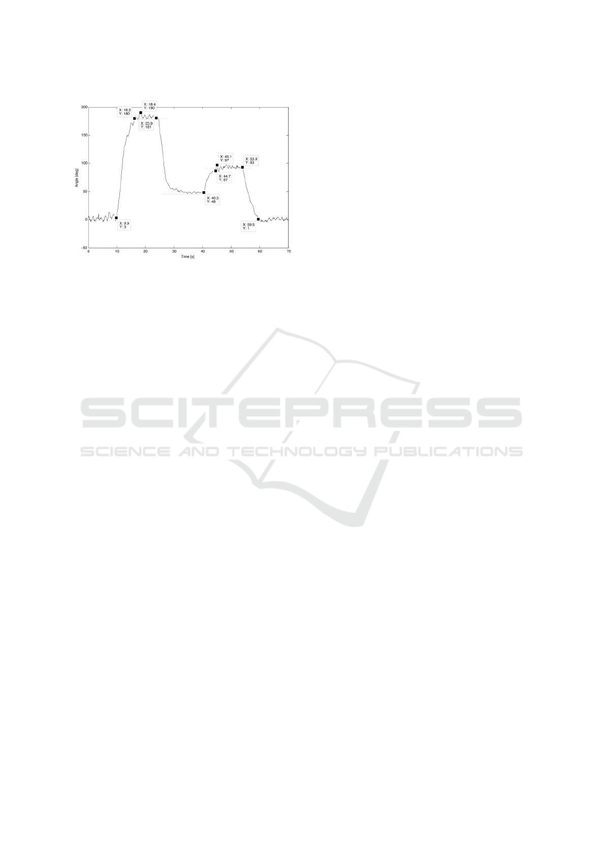
Figure 17: Performance of the auto mode controller, yaw

(Schmid, 2008).

6 DISCUSSION

6.1 System Design

The mechanical part of the µAUV

has proven to be

very robust and the propulsion system has sufﬁcient

power to propel the system. One drawback of the

thrusters is the fact that the thrusters have an insuf-

ﬁcient sealing concept. This leads to the problem

that over time water accumulates in the inside of the

thrusters. An ideal solution for hovering in the water

column is the use of a buoyancy tank. All sensors ful-

ﬁll their requirements and espescially the IMU which

outputs quaternions, even though there is a need for

a more accurate acceleration, speed and position val-

ues. Being extendable and providing a lot of compu-

tational power makes the µAUV

an ideal platform for

the purposes mentioned in section 1. Communication

via an optical link has proven to be very robust even

though the data rate should be increased in the future.

A very useful feature is the possibility to program the

system when it is fully assembled.

6.2 Identiﬁcation of System Parameters

The presented simpliﬁed model is a good start but can

be improved in the future. It is used as a ﬁrst pass at-

tempt and the results are still useful for control. The

correlated errors in Figure 8 imply an error, where re-

gression fails. The bad conditioning cannot be fully

explained by high frequency noise as hypothesised.

Regression may try to average out the errors, but the

metric and the method itself expects white noise,

uncorrelated errors. Assuming that the total mass is

constant leads to a modelling error. The thrust mod-

elling might be too simplistic for the dynamic case

because static thrust does not equal dynamic thrust.

This also impacts the thrust vs. damping force re-

sults. Another cause could be laminar ﬂow in all di-

rections except for the heave direction where turbu-

lent ﬂow might dominate due to the non-streamline

battery pack.

6.3 Controller

The simulated controller has proven to work in the

real system. A major problem is the lag of position in-

formation in surge and sway and imprecise position,

speed and acceleration data.

One of the reasons for the gap between simulation

and reality (see Section 5.4) is the simpliﬁed system

model used throughout this paper. Other possible rea-

sons could be an inaccuracy in the experiments (see

Section 4) or the fully charged battery pack which

might lead to a motor speed slightly over the theo-

retical speed.

7 CONCLUSION AND FUTURE

WORK

This paper has presented a minuscule AUV named

µAUV

. As soon as basic autonomous behavior is

implemented, the µAUV

could be tested in outside

watercourses. Its behavior in water currents would

shed light on the feasibility of the application of

µAUV

in open water. It would also be very inter-

esting to implement a controller for the µAUV

to do

a roll or a loop around the y-axis. The thrusters would

have to produce a sinusoidal force with the resonance

frequency of the system on the corresponding axis. In

any case, there are a lot of conceivable functions that

could be implemented in the future.

An interface for easily equipping the µAUV

with

new sensors could accelerate many tasks. Hull im-

provements are mainly focused on the thrusters and

the battery pack. The thrusters are the weak point in

the design concerning maximum dive depth. Due to

the thruster design, the dive depth is currently lim-

ited to approximately 2m. This together with the fact

that water accumulates in the thrusters will make a

redesign of the thrusters necessary. A possible im-

provement could be a magnetically coupled thruster.

A further step towards a streamlined hull will require

a redesign of the battery pack,

A major problem of the controller, the lag of posi-

tion information in surge and sway, could be solved

with the camera on the bottom. An algorithm for op-

tical ﬂow could be implemented to calculate the ac-

tual moving speed. Furthermore, the absolute posi-

µAUV2 - Development of a Minuscule Autonomous Underwater Vehicle

195

tion could be calculated by integrating the speed. Ad-

ditionally, optical markers on the ground of the pool

further improve the position estimate. The second

camera might be used for obstacle detection. With

this additional sensor information it would be possi-

ble to create a map of the area the AUV is moving

in.

As said before, the presented simpliﬁed model is

a good start. But e.g. the error in Figure 8, implies

that the system modell can be improved.

ACKNOWLEDGEMENTS

The project DAEDALUS is funded by the German

Space Agency (DLR, Grant number: 50NA1312)

with federal funds of the Federal Ministry of Eco-

nomics and Technology (BMWi) in accordance with

the Bundestag resolution of the German Parliament.

REFERENCES

Albiez, J., Gaudig, C., Hilljegerdes, J., and Kirchner, F.

(2015). FlatFish A compact subsea-resident inspec-

tion AUV. Unknown, 1(November).

Barngrover, C., Kastner, R., Denewiler, T., and Mills, G.

(2011). The stingray auv: A small and cost-effective

solution for ecological monitoring. In OCEANS 2011,

pages 1–8.

Bryant, S. (2002). Ice-embedded transceivers for europa

cryobot communications. IEEE Aerospace Confer-

ence Proceedings, 1(1):349–356.

Christensen, L., Kampmann, P., Hildebrandt, M., Albiez, J.,

and Kirchner, F. (2009). Hardware rov simulation fa-

cility for the evaluation of novel underwater manipula-

tion techniques. In OCEANS 2009 - EUROPE, pages

1–8.

Dowdeswell, J., Evans, J., Mugford, R., Grifﬁths, G.,

McPhail, S., Millard, N., Stevenson, P., Brandon, M.,

Banks, C., Heywood, K., Price, M., Dodd, P., Jenk-

ins, A., Nicholls, K., Hayes, D., Abrahamsen, E.,

Tyler, P., Bett, B., Jones, D., Wadhams, P., Wilkin-

son, J., Stansﬁeld, K., and Ackley, S. (2008). In-

struments and methodsautonomous underwater vehi-

cles (auvs) and investigations of the ice/ocean inter-

face in antarctic and arctic waters. Journal of Glaciol-

ogy, 54(187):661–672.

Fechner, S., Kerdels, J., Albiez, J., and Kirchner, F. (2007).

Design of a uauv. In Autonomous Minirobots for Re-

search and Edutainment (AMiRE-2007). Proceedings

of the 4th International AMiRE Symposium (AMiRE-

2007), Heinz Nixdorf Institut Universit Paderborn,

pages 99-106.

Fossen, T. I. (2002). Marine control systems: guidance,

navigation and control of ships, rigs and underwater

vehicles. Marine Cybernetics AS.

Indiveri, G. (1998). Modelling and identiﬁcation of under-

water robotic systems. Computer Science.

Kalman, R. E. (1960). A new approach to linear ﬁltering

and prediction problems. Transactions of the ASME–

Journal of Basic Engineering, 82(Series D):35–45.

Leonessa, A. (2008). Underwater robots: Motion and

force control of vehicle-manipulator systems (g. an-

tonelli; 2006) [book review]. IEEE Control Systems,

28(5):138–139.

Meyer, B., Ehlers, K., Isokeit, C., and Maehle, E. (2014).

The development of the modular hard- and software

architecture of the autonomous underwater vehicle

monsun. In ISR/Robotik 2014; 41st International

Symposium on Robotics; Proceedings of, pages 1–6.

Mintchev, S., Donati, E., Marrazza, S., and Stefanini, C.

(2014). Mechatronic design of a miniature underwater

robot for swarm operations. In Robotics and Automa-

tion (ICRA), 2014 IEEE International Conference on,

pages 2938–2943.

Nicholson, J. and Healey, A. (2008). The present state

of autonomous underwater vehicle (auv) applications

and technologies. Marine Technology Society Journal,

42(1):44–51.

Ridao, P., Batlle, J., and Carreras, M. (2001). Model identi-

ﬁcation of a low-speed uuv. IFAC Conference Control

Applications in Marine Systems, Glasgow, Scotland.

Schmid, K. (2008). Embedded system and controller

design for a micro AUV Diploma thesis. The-

sis, University of Bremen, TU Hamburg Harburg.

https://www.researchgate.net/publication/299283880

Embedded system and controller design for a

micro AUV.

Yoerger, D. and Slotine, J.-J. (1991). Adaptive sliding

control of an experimental underwater vehicle. In

Robotics and Automation, 1991. Proceedings., 1991

IEEE International Conference on, pages 2746–2751

vol.3.

ICINCO 2016 - 13th International Conference on Informatics in Control, Automation and Robotics

196