Comparison of Various Deﬁnitions of Proximity in Mixture Estimation

Ivan Nagy

1,2

, Evgenia Suzdaleva

and Pavla Pecherkov

1,2

Department of Signal Processing, The Institute of Information Theory and Automation of the Czech Academy of Sciences,

Pod vod

arenskou v

ı 4, 18208, Prague, Czech Republic

Faculty of Transportation Sciences, Czech Technical University, Na Florenci 25, 11000, Prague, Czech Republic

Keywords:

Classiﬁcation, Recursive Mixture Estimation, Proximity, Bayesian Methods, Mixture based Clustering.

Abstract:

Classiﬁcation is one of the frequently demanded tasks in data analysis. There exists a series of approaches in

this area. This paper is oriented towards classiﬁcation using the mixture model estimation, which is based on

detection of density clusters in the data space and ﬁtting the component models to them. A chosen function

of proximity of the actually measured data to individual mixture components and the component shape play

a signiﬁcant role in solving the mixture-based classiﬁcation task. This paper considers deﬁnitions of the

proximity for several types of distributions describing the mixture components and compares their properties

with respect to speed and quality of the resulting estimation interpreted as a classiﬁcation task. Normal,

exponential and uniform distributions as the most important models used for describing both Gaussian and

non-Gaussian data are considered. Illustrative experiments with results of the comparison are provided.

1 INTRODUCTION

Mixture models are a powerful class of models used

for description of multi-modal systems, which work

in different switching regimes. Detection of an ac-

tive regime is a signiﬁcant task in various applica-

tion ﬁelds such as, for example, fault detection, diag-

nostics systems, medicine, big data related problems,

etc., see, e.g., (Yu, 2012a; Yu, 2011; Yu, 2012b).

This task is often solved within (supervised) clas-

siﬁcation issues, which distribute data observed on

the described system among some categories, using

the training set of already classiﬁed data. A range of

such methods is rather wide and includes, e.g., deci-

sion trees, Bayesian classiﬁers, rule-based methods,

including fuzzy rules, neural networks, k-nearest-

neighbor classiﬁers, genetic algorithms and other

techniques. The detailed overview of these numeri-

cal techniques can be found, e.g., in sources (Larose,

2005; Han et al., 2011; Zaki and Meira, 2014; Calders

and Verwer, 2010; Zhang, 2000; Ishibuchi et al.,

2000), etc.

Unlike them, the unsupervised classiﬁcation me-

thods are directly based on clustering solutions look-

ing for data clusters in the untrained data set, such

as hierarchical and partitioning methods (centroid-,

density-based) and many others, see an overview, in

e.g., (Berkhin, 2006; Jain, 2010; Ester et al., 1996).

A separate group of such methods is created by

model-based clustering and classiﬁcation algorithms

presented e.g., by (Bouveyron and Brunet-Saumard,

2014; Zeng and Cheung, 2014; Ng and McLachlan,

2014), etc. These methods are more complex and de-

manding.

Speciﬁc methods of this type of classiﬁcation ap-

proaches are based on estimation of mixture models.

The mixture model consists of components in the

form of probability density functions (pdfs) describ-

ing individual system regimes and a model of their

switching. The mixture-based classiﬁcation starts

from some pre-speciﬁed (mostly resulted from the ini-

tial data analysis) locations of components and per-

forms a search for density clusters in the data space

with the aim of ﬁtting component models to data. The

search for the data clusters is one of the most critical

parts of the mixture estimation algorithms.

Fundamental approaches in this area mostly fo-

cus on: (i) the use of the EM algorithm (Gupta and

Chen, 2011), see, e.g., (Boldea and Magnus, 2009;

Wang et al., 2004); (ii) Variational Bayes methods

(McGrory and Titterington, 2009;

ıdl and Quinn,

2006); (iii) Markov Chain Monte Carlo (MCMC) me-

thods (Fr

uhwirth-Schnatter, 2006; Doucet and An-

drieu, 2001; Chen and Liu, 2000), often used for

mixtures of state-space models; and (iv) recursive

Bayesian estimation algorithms (K

arn

y et al., 1998;

Nagy, I., Suzdaleva, E. and Pecherková, P.

Comparison of Various Deﬁnitions of Proximity in Mixture Estimation.

DOI: 10.5220/0005982805270534

In Proceedings of the 13th International Conference on Informatics in Control, Automation and Robotics (ICINCO 2016) - Volume 1, pages 527-534

ISBN: 978-989-758-198-4

527

Peterka, 1981; K

arn

y et al., 2006; Nagy et al., 2011;

Suzdaleva et al., 2015), etc.

The present paper deals with the mixture-based

classiﬁcation using the last part of the enumerated

approaches, which is directed at algebraic computing

the statistics of the involved component distributions

avoiding applying the numerical techniques. A signi-

ﬁcant role in this process is played by the chosen func-

tion of the proximity of the actually measured data

item and individual mixture components.

This paper considers several deﬁnitions of a func-

tion used as the proximity and compares their proper-

ties with respect to speed and quality of the resulting

mixture estimation interpreted as a classiﬁcation task.

Three types of components are considered: the nor-

mal distribution as the most important type of compo-

nents, and also exponential and uniform distributions,

which are essential in modeling non-Gaussian data.

The paper is organized in the following way. The

preparative Section 2 introduces the used models and

recalls necessary basic facts about their individual re-

cursive estimation under the Bayesian methodology.

Section 3 is devoted to introducing the proximity

within the mixture estimation algorithm and its cho-

sen deﬁnitions. Section 3.4 speciﬁes the algorithm

in the uniﬁed form for all types of components and

proximity deﬁnitions. Section 4 provides results of

their experimental comparison. Conclusions and open

problems are given in Section 5.

2 MODELS

Let’s consider a multi-modal system, which at each

discrete time instant t = 1,2,.... generates the continu-

ous data vector y

. It is assumed that the observed sys-

tem works in m

working modes, each of them is indi-

cated at the time instant t by the value of the unmea-

sured dynamic discrete variable c

∈ {1,2,... ,m

which is called the pointer (K

arn

y et al., 1998).

The observed system is supposed to be described

by a mixture model, which (in this paper) consists of

components in the form of the following pdfs

f (y

|Θ,c

= i), i ∈ {1,2,. .., m

}, (1)

where Θ = {Θ

}

i=1

is a collection of unknown

parameters of all components, and Θ

includes

parameters of the i-th component in the sense that

f (y

|Θ,c

= i) = f (y

|Θ

) for c

= i.

The component, which describes data generated

by the system at the time instant t is said to be active.

2.1 Dynamic Pointer Model

Switching the active components (1) is described by

the dynamic model of the pointer

f (c

= i|c

t−1

= j,α) , i, j ∈ {1, 2,. .., m

}, (2)

which is represented by the transition table

= 1 c

= 2 ·· · c

= m

t−1

= 1 α

1|1

2|1

·· · α

t−1

= 2 α

1|2

·· ·

·· · ·· · ·· · ·· · ·· ·

t−1

= m

1|m

·· · α

where the unknown parameter α is the (m

× m

dimensional matrix, and its entries α

i| j

are non-

negative probabilities of the pointer c

= i (express-

ing that the i-th component is active at time t) under

condition that the previous pointer c

t−1

= j.

According to (K

arn

y et al., 2006), the parameter α

of the pointer model (2) is estimated using the conju-

gate prior Dirichlet pdf in the Bayes rule, recomputing

its initially chosen statistics and its normalizing.

Depending on the nature of the measured data, the

pdfs of components can be speciﬁed as follows.

2.2 Normal Components

Under assumption of normality of measurements, the

pdf (1) can be speciﬁed as

(2π)

−N/2

−1/2

exp



−

− θ

]

−1

− θ

]



, (3)

where N denotes a dimension of the vector y

; for each

i ∈ {1,2, ... ,m

} the parameter θ

represents the cen-

ter of the i-th component; r

is the covariance matrix

of the involved normal noise, which deﬁnes the shape

of the component, and here {θ

} ≡ Θ

The point estimates of parameters θ

and r

of in-

dividual components are used in computing the proxi-

mity (this will be explained later). Necessary ba-

sic facts about calculation of the point estimates are

brieﬂy given below.

According to (Peterka, 1981; K

arn

y et al., 1998),

parameters θ

and r

of the individual i-th component

(3) (omitting here for simplicity the subscript i) are

estimated via the Bayes rule using the conjugate prior

Gauss-inverse-Wishart pdf with the reproducible (ini-

tially chosen) statistics V

t−1

and k

t−1

of the appropri-

ate dimensions. The statistics are updated as follows:

= V

t−1





, 1], (4)

= κ

t−1

+ 1, (5)

ICINCO 2016 - 13th International Conference on Informatics in Control, Automation and Robotics

528

and the point estimates of parameters are respectively

= V

−1

, ˆr

−V

−1

(6)

with the help of partition V





, (7)

where V

is the square matrix of the dimension

(N × N), V

is N-dimensional column vector and V

is scalar, see details in (Peterka, 1981).

2.3 Exponential Components

The exponential distribution of components (1),

which is often suitable for situations, where the as-

sumption of normality brings a series of limitations

(non-negative, bounded data, etc.) can be speciﬁed as

∏

l=1

)

exp



−a

− b

)



, (8)

i.e., here {a

} ≡ Θ

, and (a

)

> 0 and (b

)

∈ R are

the l-th entries of the N-dimensional vectors a

and

respectively with l = {1,2 .. .,N}. Currently the

independence of entries of the vector y

is assumed.

Basic facts about the recursive estimation of the

parameters a

and b

, which are necessary to obtain

the proximity (explained later) are recalled below.

With the help of the Bayes rule and the prior expo-

nential pdf, the parameters of the individual i-th ex-

ponential component (8) are obtained, using the al-

gebraic update of the initially chosen statistics S

t−1

and B

t−1

. It is done at each time instant t as

follows (omitting here the subscript i for simplicity):

= S

t−1

+ y

, (9)

= K

t−1

+ 1, (10)

= B

l;t−1

− y

l;t

, (11)

where, denoting δ

for the l-th entry y

l;t

of y

if δ

> 0, B

l;t

= B

l;t−1

− δ

; (12)

else B

l;t

= B

l;t

+ ε, (13)

where B

l;t

is the l-th entry of the statistics B

, and ε

can be taken as 0.1. The point estimates of parameters

are obtained from

ˆa

l;t

− K

l;t

, (14)

l;t

= B

l;t

, (15)

where ˆa

l;t

and

l;t

are entries of vectors ˆa

and

re-

spectively, see, e.g., (Yang et al., 2013), and S

l;t

is the

l-th entry of the statistics S

2.4 Uniform Components

The pdf (1) with the uniform distribution often serves

as an appropriate tool for description of bounded data.

In this paper the independence of entries of the vector

is assumed, and therefore, ∀i ∈ {1, 2,.. ., m

} the

pdf (1) takes the form

f (y

|L,R, c

= i) =

(

−L

for y

∈ (L

0 otherwise,

(16)

i.e., here {L

} ≡ Θ

, and their entries (L

)

and

)

are respectively minimal and maximal bounds

of the l-th entry y

l;t

of the vector y

for the i-th uni-

form component.

The estimation of parameters of the individual i-

th uniform component (16) in the case of independent

data entries is performed using the initially chosen

statistics L

t−1

and R

t−1

with the update of their l-th

entries for each l ∈ {1,. .., N} in the following form,

see, e.g., (Casella and Berger, 2001):

if y

l;t

< L

l;t−1

, then L

l;t

= y

l;t

, (17)

if y

l;t

> R

l;t−1

, then R

l;t

= y

l;t

, (18)

where the subscript i is omitted for simplicity. The

point estimates of parameters are computed via

= L

= R

. (19)

3 PROXIMITY DEFINITIONS

3.1 General Estimation Algorithm

The mixture estimation algorithm is derived using the

joint pdf for all variables to be estimated, i.e., Θ,

α and c

, and its gradual marginalization over all of

them. In general, based on (K

arn

y et al., 1998; K

arn

et al., 2006; Peterka, 1981; Nagy et al., 2011), after

initialization, the recursive mixture estimation algo-

rithm includes the following steps at each time instant

t (here they are given only to help a reader to be ori-

ented in the discussed ﬁeld):

1. Measure new data.

2. Compute the proximity of the current data item

to each component. It is done by substituting the

measured data item and the point parameter esti-

mates from the previous time instant into corre-

sponding components.

3. Construct the weighting vector containing the

probabilities of the activity of components at the

actual time instant. It is obtained by using the ob-

tained proximities, the prior pointer pdf and the

previous point estimate of α.

Comparison of Various Deﬁnitions of Proximity in Mixture Estimation

529

4. Update the statistics of all components using the

weighting vector, and statistics of the pointer

model, using the weighting matrix joint for the

current pointer c

and the previous one c

t−1

5. Recompute the point estimates of all parameters

and then use them as the initial ones in the ﬁrst

step of the on-line algorithm.

More detailed information can be also found in (Suz-

daleva et al., 2015).

3.2 Proximity as the Approximated

Likelihood

The proximity appeared in Step 2 of the above algo-

rithm is explained in this section. Originally, accord-

ing to (K

arn

y et al., 2006) the proximity has been in-

troduced for the normal distribution as the likelihood

for different variants of the model – as the so-called

v-likelihood. In the considered context the variants of

the normal distribution are given by normal compo-

nents (3) labeled by the pointer value c

= i. Gener-

ally the proximity is derived based on the following

scheme. For each i ∈ {1,2,. .. , m

} under assumption

of the mutual independence of Θ and α, and y

and α,

and c

and Θ it takes the form

f (Θ,c

= i,c

t−1

= j,α|y(t))

| {z }

joint posterior pd f

∝ f (y

,Θ, c

= i,c

t−1

= j,α|y(t − 1))

| {z }

via the chain rule and Bayes rule

= f (y

|Θ,c

= i)

{z }

(1)

f (Θ|y(t − 1))

| {z }

prior pd f o f Θ

× f (c

= i|α,c

t−1

= j)

| {z }

(2)

f (α|y(t − 1))

| {z }

prior pd f o f α

× f (c

t−1

= j|y(t − 1)),

{z }

prior pointer pd f

(20)

where y(t) = {y

,. .. ,y

} represents the collection

of data available up to the time instant t, and y

de-

notes the prior knowledge. With the help of integrals

of (20) over Θ, α and summation over c

t−1

, the v-

likelihood denoted by L

for the pointer value c

= i

is obtained as

= i|y(t − 1)) =

∑

t−1

∗

f (y

|Θ,c

= i)

| {z }

(1)

× f (Θ|y(t − 1))

| {z }

prior pd f o f Θ

f (c

= i|α,c

t−1

= j)

| {z }

(2)

× f (α|y(t − 1))

| {z }

prior pd f o f α

f (c

t−1

= j|y(t − 1))

| {z }

prior pointer pd f

dΘ dα. (21)

The considered approximation via the Dirac delta

function consists in substituting the point estimates of

parameters Θ

and α into (21), which gives

= i|y(t − 1))

= f



i;t−1

= i



× f



= i|

i| j;t−1

t−1

= j



, (22)

where

i;t−1

is the point estimate of Θ from the pre-

vious time instant t − 1, and

i| j;t−1

is the entry of

the point estimate

t−1

at time t − 1. Thus, the re-

sult (22) is the predictive pdf existing for each i, j ∈

{1,2, .. .,m

} with the substituted current data item y

and the available parameter point estimates. This pdf

is deﬁned as the proximity of the actual data item and

the i-th component.

For normal components (3) the predictive pdf has

the Student distribution. It is chosen as one of deﬁ-

nitions of the proximity to be used during the recur-

sive mixture estimation.

3.3 Proximity as Decreasing Functions

Distinguishing the individual components is a compli-

cated part of the mixture estimation. The used proxi-

mity can unambiguously assign the measured data

item (if possible) to one of the components. Since

components in the data space can be of a different

shape and located on a different distance from each

other, and also with a variously decreasing density of

data items on their edges, it is important to choose a

suitable distance measure. This is determined by the

chosen deﬁnition of the proximity.

The main requirement for the proximity function

is to be at its maximum at the center of a component

and to decrease rapidly with the increasing distance.

The speed of decreasing should be fast enough. That’s

is why it is advantageous to apply the proximity func-

tion with a curve of the normal distribution.

Other functions also have similar properties and

thus can be explored as the proximity. Generally a

power function can decrease in the beginning of its

course faster than an exponential function, but at a

larger distance the exponential function is closer to

zero. Comparison of these functions as the proximity

is the main task of the presented research.

Based on this idea, different deﬁnitions of the

proximity can be chosen using a rapidly decreasing

function depending on

∆

= y

− E[y

], (23)

where the expectation E[y

] is computed for the cor-

responding type of components.

For the i-th normal component (3) the expectation

is given by the point estimate of θ

according to (6).

ICINCO 2016 - 13th International Conference on Informatics in Control, Automation and Robotics

530

For the i-th exponential component the expecta-

tion can be obtained as

( ˆa

l;t−1

)

+ (

l;t−1

)

(24)

using the point estimates (14)–(15) for the l-th entries

of the vector y

For the i-th uniform component the expectation is

a simple average of the component bounds L

and R

for corresponding entries of the vector y

Using ∆

from (23) the following rapidly de-

creasing functions (as combinations of the mentioned

above) are considered:

1. The polynomial of the form

1/∆

. (25)

2. The normal approximation of other distributions,

optimal in the sense of the Kullback-Leibler diver-

gence, see, e.g., (K

arn

y et al., 2006), which is the pdf

(3) with the substituted expectation of the correspond-

ing type of the components instead of θ

. The covari-

ance matrices can be either used from individual dis-

tributions or chosen as the diagonal ones in case only

the expectations should be estimated.

3. The polynomial in the form

exp{−(2∆

)

}. (26)

4. The Student distribution based relation



1 +

∆



−

. (27)

3.4 Algorithm

The mixture estimation algorithm tailored to the

above proximity deﬁnitions is summarized as follows.

Initialization (for t=1)

• Set the number of components m

• Set the initial statistics for the corresponding type

of components, i.e., either for (3) or (8), or (16),

see Section 2.

• Set the initial Dirichlet statistics of the pointer

model (2) according to (K

arn

y et al., 2006) as the

× m

)-dimensional matrix denoted by γ

• Using the initial statistics, compute the initial

point estimates of parameters of all components

using either (6) or (14)–(15), or (19).

• Compute the initial point estimate of α by norma-

lizing the Dirichlet statistics γ

• Set the initial m

-dimensional weighting vector

On-line part (for t=2,. . . )

1. Measure the new data item y

2. Compute the expectations E[y

] of all components

using the corresponding point estimates.

3. For all components, obtain (23) by substituting y

and the expectations E[y

4. For all components, substitute the obtained ∆

into

the chosen type of the proximity, i.e., either (25),

(3), (26) or (27).

5. In each case the result is the m

-dimensional vec-

tor of proximities, which has one entry for each

component. These entries are proportional to the

inverse distance of the data item to the individual

components. The higher the number is, the closer

the data item is to the component.

6. Multiply entry-wise the resulted vector from the

previous step, the previous weighting vector w

t−1

and the previous point estimate of α. The result of

the multiplication is the matrix of weights denoted

by W

i, j;t

joint for c

and c

t−1

7. Perform the summation of the normalized matrix

from the previous step over rows and obtain the

updated weighting vector w

. The maximal entry

of the weighting vector gives the point estimate of

the pointer c

, i.e., the currently active component.

8. For all components, update the statistics with the

help of multiplying the data-dependent increment

in each statistics by the corresponding entry from

the actualized weighting vector w

, see (K

arn

y et

al., 1998; K

arn

y et al., 2006; Peterka, 1981; Nagy

et al., 2011; Suzdaleva et al., 2015; Nagy et al.,

2016).

9. Update the statistics of the pointer model as

i| j;t

= γ

i| j;t−1

i, j;t

(28)

based on (K

arn

y et al., 1998; Nagy et al., 2011).

10. Recompute the point estimates of all parameters

and use them for Step 1 of the on-line part.

4 EXPERIMENTS

This section provides the experimental comparison

of evolution of the proximities (25), (3), (26) and

(27) for all three discussed types of components ac-

cording to the above algorithm. The simulated two-

dimensional data were used, which is quite sufﬁcient

for adequate judging the proximity evolution. Three

components of each type were simulated. A series of

experiments with the various number of data was per-

formed. Here typical results are demonstrated.

Comparison of Various Deﬁnitions of Proximity in Mixture Estimation

531

The quality of classiﬁcation as the detection of the

active component at each time instant according to the

maximal weights was compared. Firstly, easily distin-

guishable components as a simple case were tested.

Results for them are provided in Table 1. Then, a

case with two components closer to each other and

the third at a larger distance was tested, see Table 2.

Finally, the most complicated case with overlapped

components was tested, see results in Table 3.

Table 1: Average number of incorrect pointer point esti-

mates (%) for easily distinguishable components.

Proximities / components (3) (8) (16)

1/∆

1.2 0 3.4

Approximation (3) 0 65.5 0.4

exp{−(2∆

)

} 0 0 0.4



1 +

∆



−

26.4 0 0.4

Table 2: Average number of incorrect pointer point esti-

mates (%) for variously located components.

Proximities / components (3) (8) (16)

1/∆

7.4 6.6 15.8

Approximation (3) 27.2 67.4 11.2

exp{−(2∆

)

} 15.8 3.6 11.2



1 +

∆



−

21.4 4.6 12

Table 3: Average number of incorrect pointer point esti-

mates (%) for overlapped components.

Proximities / components (3) (8) (16)

1/∆

39.4 39.2 19.2

Approximation (3) 37.8 67.4 15.4

exp{−(2∆

)

} 39.6 33.4 15.4



1 +

∆



−

39.2 37.2 16

These tables brieﬂy (due to a lack of space)

present results of comparison. Nevertheless, to sum-

marize results obtained for variously noised data (that

determines distances among components) the follow-

ing trend is observed.

For easily distinguishable components all the

proximity deﬁnitions are similarly successful with the

insigniﬁcant difference, excepting the Student distri-

bution based function (27) for normal components,

and the normal approximation of the exponential dis-

tributions.

Variously located components, where two compo-

nents are closer to each other and the third is at a

larger distance, is a more challenging task. In this

case the trend in success of classiﬁcation of exponen-

tial and uniform components is preserved. However,

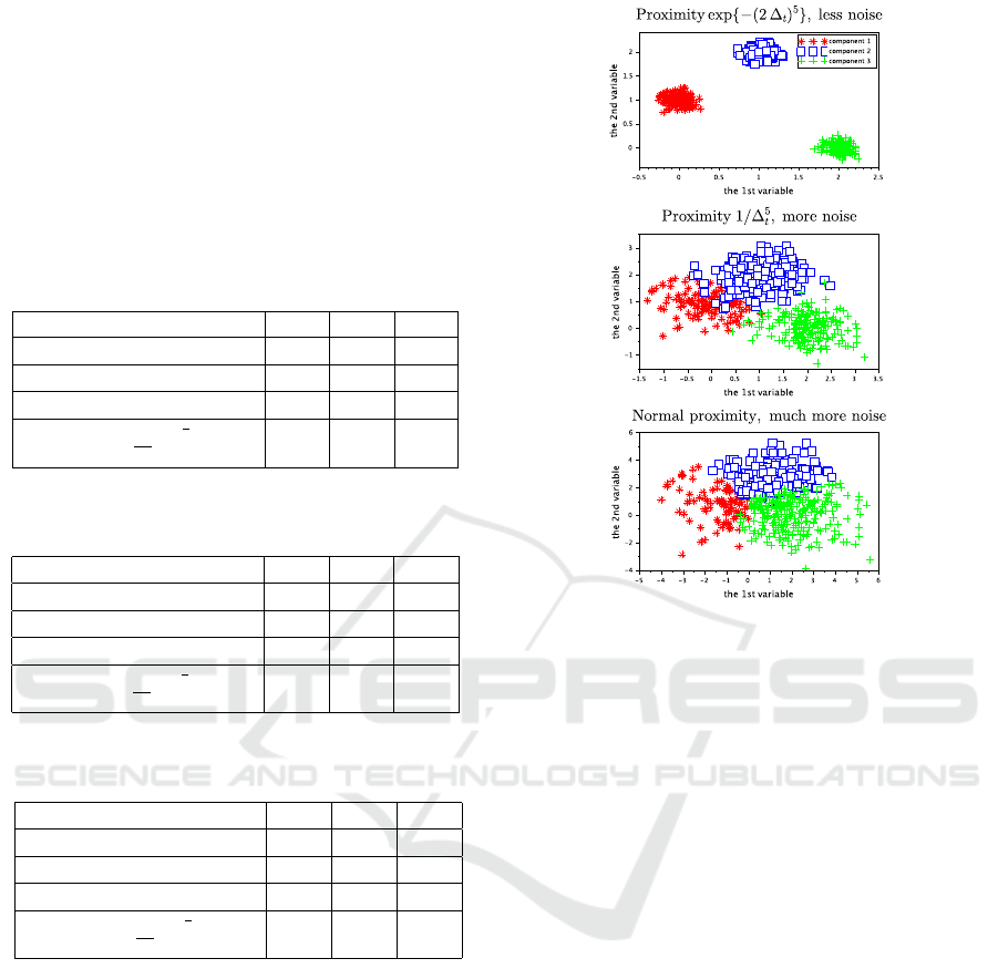
Figure 1: The most successful classiﬁcation results with

normal components from Tables 1, 2 and 3.

signiﬁcant worsening can be seen for the proximity

(3) for normal components. The proximity 1/∆

gives

the best results.

For strongly overlapped components (which is the

most complicated and also realistic case) the situation

changes. For normal components all results are simi-

lar, but now the proximity deﬁnition (3) is the most

successful.

It seems that a decision about a choice of the

proximity deﬁnition is suitable to make in accordance

to the noise covariance matrix estimation. For the less

noised data the distance-based proximities 1/∆

and

exp{−(2∆

)

} can be used. The normal approxima-

tion (3) is not suitable for exponential components,

but it can be used for uniformed components. For

more noised data the normal approximation (3) can

be used both for normal and uniform components.

The graphical presentation of the classiﬁcation re-

sults is given for normal components in Figure 1,

where (due to a lack of space) the most successful

combinations of the proximity deﬁnition and a dis-

tance among components are shown. In all ﬁgures

three detected components are sharply visible.

Selected results for exponential components can

be seen in Figure 2, where the evolution of the com-

ponent centers during the on-line estimation is plotted

for the proximity (26) (top) and (27) (bottom). The

ICINCO 2016 - 13th International Conference on Informatics in Control, Automation and Robotics

532

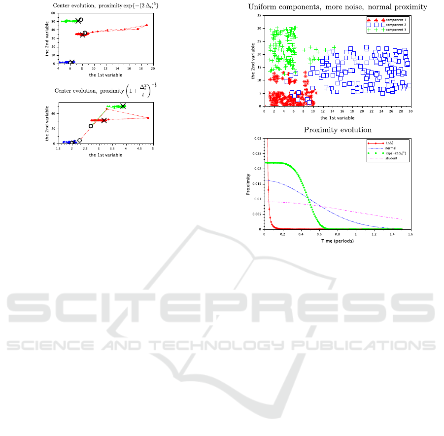
Figure 2: Evolution of exponential component centers du-

ring the estimation with the proximity exp{−(2∆

)

} (top)

and the Student based proximity (bottom).

initial centers are denoted by the circle, the ﬁnal – by

’x’. The ﬁgures show that although the success of the

estimation according to Table 1 were the same for the

proximity (26) and (27), the stabilization of compo-

nent centers took a different time. In the top ﬁgure the

centers were correctly located just in the beginning of

estimation, while in the bottom ﬁgure the search for

correct locations was performed a bit longer.

For uniform components the classiﬁcation results

were close to each other for all tested types of loca-

tion of components. It is worth noting that the nor-

mal approximation (3) and the distance-based proxi-

mity (26) were similarly successful. Results with one

of them for variously located components are demon-

strated in Figure 3 (top).

The proximity evolution during the chosen time

interval is shown in Figure 3 (bottom). The distance-

based proximity 1/∆

demonstrates the strongest

sharpness. The normal approximation has a smoother

course. The third proximity from Table 1 is in-

ﬂuenced by the constant, which allows to move its

course as necessary. The Student distribution based

proximity is close to ﬂat.

5 CONCLUSIONS

The aim of the described recursive classiﬁcation is the

analysis of real data in real time, which suggests that

the detected clusters can be of various shapes. Thus

solutions with mixtures of different components are

highly desired.

Using the point estimates directly in the exponen-

tial and uniform models as the proximity gives unsuc-

cessful results during the mixture estimation, which

can be explained by asymmetric distributions. One

Figure 3: Detected uniform components with the proximity

(3) (top) and the proximity evolution for a selected interval

(bottom).

of the attempts was the use of the normal approxima-

tion optimal from the point of view of the Kullback-

Leibler divergence. The important property of the

proximity is its rapidly decreasing course. This is sat-

isﬁed by the normal approximation, but other func-

tions can be also relevant for the considered task. The

results of the comparison show that for different types

of components a choice of the proximity is not un-

ambiguous and inﬂuences the classiﬁcation results.

Thus, the signiﬁcance of the proximity choice is con-

ﬁrmed.

However, there is still a series of open problems

in this area, including (i) the solution for dependent

entries of the data vector for exponential and uniform

distributions, (ii) extension of the recursive mixture

estimation theory for other distributions describing

non-Gaussian data, and (iii) classiﬁcation with a mix-

ture of different distributions. This will be the plan of

the future work within the present project.

ACKNOWLEDGEMENTS

The paper was supported by project GA

CR GA15-

03564S.

Comparison of Various Deﬁnitions of Proximity in Mixture Estimation

533

REFERENCES

Yu, J. (2012). A nonlinear kernel Gaussian mixture model

based inferential monitoring approach for fault detec-

tion and diagnosis of chemical processes, Chemical

Engineering Science, vol. 68, 1, p. 506–519.

Yu, J. (2012). A particle ﬁlter driven dynamic Gaussian

mixture model approach for complex process moni-

toring and fault diagnosis, Journal of Process Control,

vol. 22, 4 , p. 778–788.

Yu, Jianbo. (2011). Fault detection using principal

components-based Gaussian mixture model for semi-

conductor manufacturing processes, IEEE Transac-

tions on Semiconductor Manufacturing, vol. 24, 3, p.

432–444.

Larose, D. T. (2005). Discovering Knowledge in Data. An

Introduction to Data Mining. Willey.

Han, J., Kamber, M., Pei, J. (2011). Data Mining: Con-

cepts and Techniques, 3rd ed. (The Morgan Kaufmann

Series in Data Management Systems). Morgan Kauf-

mann.

Zaki, M.J., Meira Jr.. W. (2014). Data Mining and Anal-

ysis: Fundamental Concepts and Algorithms. Cam-

bridge University Press.

Calders, T., Verwer, S. (2010). Three naive Bayes ap-

proaches for discrimination-free classiﬁcation. Data

Mining and Knowledge Discovery. 21(2), p. 277–292.

Zhang, G. P. (2000). Neural Networks for Classiﬁcation:

A Survey. In: IEEE Transactions on System, Man,

and Cybernetics – Part C: Applications and Reviews.

30(4), November, p. 451–462.

Ishibuchi, H., Nakashima, T., Nii, M. (2000). Fuzzy If-Then

Rules for Pattern Classiﬁcation. In: The Springer In-

ternational Series in Engineering and Computer Sci-

ence. 553, p. 267–295.

Berkhin, P. (2006). A Survey of Clustering Data Mining

Techniques. In: Grouping Multidimensional Data.

Eds.: J. Kogan, C. Nicholas, M. Teboulle. Springer

Berlin Heidelberg, p.25–71.

Jain, A. K. (2010). Data clustering: 50 years beyond K-

means. Pattern Recognition Letters. 31(8), p. 651–

666.

Ester, M., Kriegel, H.-P., Sander, J., Xu, X. (1996). A

density-based algorithm for discovering clusters in

large spatial databases. In: Proc. 1996 Int. Conf.

Knowledge Discovery and Data Mining (KDD’96),

Portland, OR, August, p. 226–231.

Bouveyron, C., Brunet-Saumard, C. (2014). Model-based

clustering of high-dimensional data: A review. Com-

putational Statistics & Data Analysis. 71(0), p. 52–78.

Zeng, H., Cheung, Y. (2014). Learning a mixture model

for clustering with the completed likelihood minimum

message length criterion. Pattern Recognition. 47(5),

p. 2011–2030.

Ng, S.K., McLachlan, G.J. (2014). Mixture models for clus-

tering multilevel growth trajectories. Computational

Statistics & Data Analysis. 71(0), p. 43–51.

Gupta, M. R. , Chen, Y. (2011). Theory and use of the EM

method. In: Foundations and Trends in Signal Pro-

cessing, vol. 4, 3, p. 223–296.

Boldea, O., Magnus, J. R. (2009). Maximum likelihood

estimation of the multivariate normal mixture model,

Journal of The American Statistical Association, vol.

104, 488, p. 1539–1549.

Wang, H.X., Luo, B., Zhang, Q. B., Wei, S. (2004). Estima-

tion for the number of components in a mixture model

using stepwise split-and-merge EM algorithm, Pattern

Recognition Letters, vol. 25, 16, p. 1799–1809.

McGrory, C. A., Titterington, D. M. (2009). Variational

Bayesian analysis for hidden Markov models, Aus-

tralian & New Zealand Journal of Statistics, vol. 51,

p. 227–244.

ıdl, V., Quinn, A. (2006). The Variational Bayes Method

in Signal Processing, Springer-Verlag Berlin Heidel-

berg.

uhwirth-Schnatter, S. (2006). Finite Mixture and Markov

Switching Models, Springer-Verlag New York.

Doucet, A., Andrieu, C. (2001). Iterative algorithms for

state estimation of jump Markov linear systems. IEEE

Transactions on Signal Processing, vol. 49, 6, p.

1216–1227.

Chen, R., Liu, J.S. (2000). Mixture Kalman ﬁlters. Journal

of the Royal Statistical Society: Series B (Statistical

Methodology), vol. 62, p. 493–508.

arn

y, M., Kadlec, J., Sutanto, E.L. (1998). Quasi-Bayes

estimation applied to normal mixture, In: Preprints

of the 3rd European IEEE Workshop on Computer-

Intensive Methods in Control and Data Processing

(eds. J. Roj

cek, M. Vale

ckov

a, M. K

arn

y, K. War-

wick), CMP’98 /3./, Prague, CZ, p. 77–82.

Peterka, V. (1981). Bayesian system identiﬁcation. In:

Trends and Progress in System Identiﬁcation (ed. P.

Eykhoff), Oxford, Pergamon Press, 1981, p. 239–304.

arn

y, M., B

ohm, J., Guy, T. V., Jirsa, L., Nagy, I., Ne-

doma, P., Tesa

r, L. (2006). Optimized Bayesian Dy-

namic Advising: Theory and Algorithms, Springer-

Verlag London.

Nagy, I., Suzdaleva, E., K

arn

y, M., Mlyn

rov

a, T. (2011).

Bayesian estimation of dynamic ﬁnite mixtures. Int.

Journal of Adaptive Control and Signal Processing,

vol. 25, 9, p. 765–787.

Suzdaleva, E., Nagy, I., Mlyn

rov

a, T. (2015). Recursive

Estimation of Mixtures of Exponential and Normal

Distributions. In: Proceedings of the 8th IEEE In-

ternational Conference on Intelligent Data Acquisi-

tion and Advanced Computing Systems: Technology

and Applications, Warsaw, Poland, September 24–26,

p.137–142.

Yang, L., Zhou, H., Yuan, H. (2013). Bayes Estima-

tion of Parameter of Exponential Distribution under

a Bounded Loss Function. Research Journal of Math-

ematics and Statistics, vol.5, 4, p.28–31.

Casella, G., Berger R.L. (2001). Statistical Inference, 2nd

ed., Duxbury Press.

Nagy, I., Suzdaleva, E., Mlyn

rov

a, T. (2016). Mixture-

based clustering non-gaussian data with ﬁxed bounds.

In: Proceedings of the IEEE International conference

Intelligent systems IS’16, Soﬁa, Bulgaria, September

4–6, accepted.

ICINCO 2016 - 13th International Conference on Informatics in Control, Automation and Robotics

534