On Nonlinearity Measuring Aspects of Stochastic Integration Filter

Jind

rich Havl

ık, Ond

rej Straka, Jind

rich Dun

ık and Ji

ı Ajgl

European Centre of Excellence - New Technologies for Information Society,

Department of Cybernetics, University of West Bohemia, Technick

a 8, Pilsen, Czech Republic

Keywords:

State Estimation, Bayesian Approach, Stochastic Integration, Measures of Nonlinearity, Measures of

Non-Gaussianity.

Abstract:

The paper deals with Bayesian state estimation of nonlinear stochastic dynamic systems. The focus is aimed at

the stochastic integration ﬁlter, which is based on a stochastic integration rule. It is shown that the covariance

matrix of the integration error calculated as a byproduct of the rule can be used as a measure of nonlinearity.

The measure informs the user about validity of the assumptions of Gaussianity, which is adopted by the

stochastic integration ﬁlter. It is also demonstrated how to use this information for a prediction of the number

of remaining iterations of the rule. The paper also focuses on utilization of the integration error covariance

matrix for improving estimates of the mean square error of the estimates, which is produced by the ﬁlter.

1 INTRODUCTION

Nonlinear state estimation of discrete-time stochas-

tic dynamic systems is an important ﬁeld of study,

which has undergone a rapid development in the last

two decades. The importance of this ﬁeld stems from

its crucial role in many areas such as signal process-

ing, target tracking, satellite navigation, fault detec-

tion, and adaptive and optimal control problems. It is

an essential part of any decision-making process.

The system state completely characterizes the sys-

tem at a given time and usually is not directly measur-

able. The system behavior is described by a stochastic

dynamic discrete-time model consisting of a stochas-

tic difference equation characterizing dynamics of the

state and by a stochastic algebraic equation represent-

ing a relation between the state and the measurement.

The solution to the state estimation problem usually

follows the Bayesian approach or the optimization ap-

proach.

The Bayesian approach is built up on the Bayesian

recursive relations (BRRs) (Sorenson, 1974), which

provide the state estimate in the form of a conditional

probability density function (PDF) of the state condi-

tioned by the measurement. However, the exact solu-

tion to the BRRs can be found only for a few special

cases, such as a linear system with Gaussian distur-

bances. For a nonlinear or non-Gaussian system the

conditional PDF has a complex shape and the solu-

tion usually cannot be found in a closed form. Hence,

some approximations must be employed.

A group of approximate methods providing ap-

proximate conditional PDF capturing the complexity

of the conditional PDF with a great ﬁdelity are called

global methods. They are represented namely by the

Gaussian sum method (Ristic et al., 2004), the point-

mass method (Kramer and Sorenson, 1988), and the

particle ﬁlter (Doucet et al., 2001). The practical use

of the global methods is limited especially due to their

extensive computational complexity.

Another group of methods is formed by assum-

ing Gaussian approximation of the conditional PDF

provided by the BRRs. Such methods are denoted as

Gaussian ﬁlters (GFs) (Ito and Xiong, 2000) or local

Bayesian methods (Arasaratnam and Haykin, 2009).

The GFs are represented namely by the quadrature

Kalman ﬁlter (Arasaratnam et al., 2007), the cuba-

ture Kalman ﬁlter (Arasaratnam and Haykin, 2009),

and the stochastic integration ﬁlter (SIF) (Dun

ık et al.,

2013b), which utilizes the iterative stochastic integra-

tion rule (SIR) (Genz and Monahan, 1998).

Contrary to the Bayesian approach, the optimiza-

tion approach assumes minimization of a certain de-

sign criterion, usually the mean square error (MSE),

leading to ﬁlters such as the extended Kalman ﬁlter,

the divided difference ﬁlter (Nørgaard et al., 2000),

or the unscented Kalman ﬁlter (Julier and Uhlmann,

2004). The optimization is usually feasible by enforc-

ing a linear structure of the ﬁlter.

Even though optimization methods and local

Bayesian methods were derived by different ap-

proaches, ﬁnally they provide formally same solution

Havlík, J., Straka, O., Duník, J. and Ajgl, J.

On Nonlinearity Measuring Aspects of Stochastic Integration Filter.

DOI: 10.5220/0005983903530361

In Proceedings of the 13th International Conference on Informatics in Control, Automation and Robotics (ICINCO 2016) - Volume 1, pages 353-361

ISBN: 978-989-758-198-4

353

to the state estimation problem, which is computa-

tionally reasonable and therefore often used in prac-

tice.

The GFs perform well only for mildly nonlinear

functions, for which the Gaussianity assumption is

approximately valid. For strong nonlinearities the

assumption is only a rough approximation. During

the last decade several methods quantifying nonlin-

earity or non-Gaussianity, which have been applied

in monitoring the GF assumption validity, have ap-

peared (Mallick, 2004), (Li, 2012) and (Dun

ık et al.,

2013a). Such methods are usually based on eval-

uating effects of nonlinearities in neighborhoods of

conditional means or testing unimodal or non-heavy-

tailed properties of the conditioned PDFs.

The goal of the paper is to show that the SIF based

on SIRs possesses nonlinearity measuring capabilities

itself. The information can be used to give the user

an idea how strong nonlinear behavior the system ex-

hibits or how much the Gaussian assumption is vio-

lated and how much the estimates should be trusted.

Further, it will be shown that the information can be

utilized to predict computational requirements of the

SIRs employed by the ﬁlter to achieve a desired ac-

curacy. And above all, the information will be used

to make the estimate of the MSE provided by the SIF

more precise.

The rest of the paper is organized as follows: Sec-

tion 2 is devoted to a brief introduction to the nonlin-

ear state estimation, its solution by the GFs, and mea-

sures of nonlinearity and non-Gaussianity. The SIR is

brieﬂy presented in Section 3. Section 4 presents the

revealed capability of the SIF to measure nonlinearity

and its application. Next, in Section 5 the utilization

of this information to provide an improved estimate

of the MSE is outlined and the paper is concluded by

Section 6.

2 STATE ESTIMATION AND

GAUSSIAN FILTERS

The aim of this section is to formulate the nonlin-

ear state estimation problem, to present its general

solution by means of the BRR, to describe the GFs,

and to present two measures of nonlinearity and non-

Gaussianity proposed in literature.

2.1 Formulation of the Nonlinear State

Estimation Problem

Let a discrete-time nonlinear stochastic system be

considered in the following state-space form

k+1

= f

) + w

, k = 0, 1,2,. . ., (1)

= h

) + v

, k = 0, 1,2,. . ., (2)

where the vectors x

∈ R

, and z

∈ R

repre-

sent the state of the system, and the measurement at

time instant k, respectively, f

: R

→ R

and h

→ R

are known vector functions, and w

∈ R

are mutually independent state and mea-

surement white noises. The PDFs of the noises are

Gaussian with zero means and known covariance ma-

trices (CMs) Σ

and Σ

, respectively, i.e., p(w

) =

N {w

×1

,Σ

}

and p(v

) = N {v

×1

,Σ

}, re-

spectively, where 0

a×b

denotes an a × b matrix of

zeros. The PDF of the initial state is Gaussian and

known as well, i.e., p(x

) = N {x

;

}. The ini-

tial state is independent of the noises.

State estimation aims at searching the state x

based on measurements up to the time instant `, which

will be denoted as z

= [z

,. . ., z

]

. Due to the

stochastic nature of the system, the state estimate is

described by the conditional PDF p(x

). In this

paper, the ﬁltering (k = `) and the one-step prediction

(k = ` + 1) problems will be considered only.

To ﬁnd the ﬁltering estimate p(x

) the Bayesian

approach is used, and the following BRRs provide the

solution (Sorenson, 1974):

p(x

) =

p(x

k−1

)p(z

)

p(x

k−1

)p(z

)dx

, (3)

where the one-step prediction PDF is

p(x

k−1

) =

p(x

k−1

)p(x

k−1

)dx

k−1

, (4)

and p(x

k−1

) = p

k−1

− f

k−1

)) and

p(z

) = p

− h

)).

An analytical solution to (3) and (4) is an intri-

cate functional-domain problem. It can be analyti-

cally computed for a few cases only. Such a case

is given by linear functions and Gaussian PDFs in

the system equations (1) and (2). So, for a nonlin-

ear or a non-Gaussian system, approximate solutions

are mostly necessary.

2.2 Gaussian Filters

The GFs suppose that the joint prediction PDF

p(z

k−1

) is at each time instant Gaussian

(Arasaratnam and Haykin, 2009)

p(z

k−1

) = N







;

k|k−1



k|k−1



(5)

For the sake of simplicity all PDFs will be given by their

argument, if not stated otherwise, i.e., p(w

) = p

ICINCO 2016 - 13th International Conference on Informatics in Control, Automation and Robotics

354

Then the ﬁltering PDF p(x

) and the one-step pre-

dictive PDF p(x

k−1

) are also Gaussian

p(x

) = N {x

;

k|k

}, (6)

p(x

k−1

) = N {x

;

k|k−1

}. (7)

The GFs compute the ﬁrst two moments of (6) and

(7), i.e., the conditional means

k|k

= E[x

] and

k|k−1

= E[x

k−1

] and the conditional CMs P

k|k

cov[x

] and P

k|k−1

= cov[x

k−1

The GF algorithm can be written in the following

form:

Algorithm 1: Gaussian Filter.

Step 1: (initialization) Set the time instant k = 0 and

deﬁne a priori initial condition by its ﬁrst two moments

0|−1

, E[x

] =

, (8)

0|−1

, E[(x

−

0|−1

)(x

−

0|−1

)

] = P

. (9)

Step 2: (ﬁltering, measurement update) The ﬁltering

mean

k|k

and CM P

k|k

are computed by the means of

k|k

k|k−1

+ K

−

k|k−1

), (10)

k|k

= P

k|k−1

− K

k|k−1

, (11)

where

= P

k|k−1

)

−1

(12)

is the ﬁlter gain and the measurement prediction

k|k−1

is given by

k|k−1

= E[z

k−1

]. (13)

The predictive CMs P

k|k−1

and P

k|k−1

are computed as

k|k−1

= E[(z

−

k|k−1

)(z

−

k|k−1

)

k−1

]

= E[(h

) −

k|k−1

)

× (h

) −

k|k−1

)

k−1

] + Σ

, (14)

k|k−1

= E[(x

−

k|k−1

)(z

−

k|k−1

)

k−1

]. (15)

Step 3: (prediction, time update) The predictive mean

k+1|k

and CM P

k+1|k

are given by

k+1|k

= E[x

k+1

] = E[f

)|z

], (16)

k+1|k

= E[(x

k+1|k

−

k+1|k

)(x

k+1|k

−

k+1|k

)

]

= E[(f

) −

k+1|k

)(f

) −

k+1|k

)

]

+ Σ

. (17)

Let k = k + 1.

The algorithm then continues by Step 2.

The particular GFs vary in the way they compute

the integrals determining the predictive characteristics

of the measurement (13-15) and the predictive char-

acteristics of the state (16, 17). Mostly, the integrals

cannot be calculated analytically. For example, the in-

tegrals can be approximated by the SIR, which leads

to the SIF.

2.3 Measures of Nonlinearity and

Non-Gaussianity

The GFs are designed under the Gaussianity assump-

tion (5), which will become invalid due to the non-

linearities present in the system. This may conse-

quently severely degrade the performance of the ﬁl-

ter, disrupt its accuracy or credibility. Hence, it is

convenient to monitor working conditions of the ﬁl-

ter, which affect validity of the assumption. For this

purpose the measures of nonlinearity (MoNL) or non-

Gaussianity (MoNG) render an applicable tool. The

MoNL and MoNG may be used for sequential moni-

toring of the GF assumption and an impact of approx-

imations along a trajectory of the GF.

Two examples of MoNL, which will be later used

for a comparison, are described below. The described

MoNL evaluate the nonlinearity of a function y =

g(x), where x is a random variable with a mean

x and

a CM P

deﬁning a region, where the nonlinearity

will be analyzed. The MoNL can be used in the ﬁl-

tering or the predictive step of the GF (Algorithm 1).

In the ﬁltering step the function g(x) is equal to is

), i.e., g(x) = h

), and in the predictive step

g(x) = f

Differential Geometry Measure based MoNL

The MoNL based on a differential geometry mea-

sure (DGM) was originally proposed in (Bates and

Watts, 1988) for the nonlinear parameter estimation

and later it was extended for the nonlinear state esti-

mation (Mallick, 2004). The MoNL directly assesses

the curvature

of the nonlinear function at a given

point. The state-independent version of the measure

is deﬁned as

MoNL

DGM

, (18)

where X

∈ R

, {X

}

i=1

is a set of q user-deﬁned

points somehow respecting the probabilistic descrip-

tion of x ,

G =

∂g(x)

∂x

is the Jacobian of g(x), and

G =

∂

g(x)

∂x∂x

is the Hessian of g(x).

Therefore, the measure assesses the contribution

of the Taylor series expansion (TSE) second order

Amount by which a curve deviates from a tangent

(hyper-)plane.

On Nonlinearity Measuring Aspects of Stochastic Integration Filter

355

term

relative to the TSE ﬁrst order term which de-

ﬁnes the tangential (linear) approximation of the func-

tion. The measure (18) can be evaluated at multiple

points X

and, its maximum can be selected for as-

sessing nonlinearity of g(x), i.e.,

MoNL

DGM

= max

i∈{1,2,...,q}

MoNL

DGM

. (19)

Least-Squares based MoNL

In (Dun

ık et al., 2013a) the weighted least-squares

(WLS) based MoNL was proposed assessing the

WLS residue, i.e., the difference between the nonlin-

ear function and its linear (least-squares) approxima-

tion deﬁned by parameters

∗

= argmin

(Y − Xθ)

W(Y − Xθ), (20)

where X =



,..., X

]

1,. . ., 1



, Y = [Y

,..., Y

]

, Y

g(X

),∀i, X

∈ R

, Y

∈ R

, {X

}

i=1

is a set of user-

deﬁned points, and W is a diagonal weighting ma-

trix respecting placement of the points X

. Then, the

MoNL is given by

MoNL

WLS

= Y

[W − WX(X

WX)

−1

W]Y.

(21)

The points {X

}

i=1

are suitably selected (user-

deﬁned) weighted points to represent the probabilistic

description of x. The largest element can be selected

for assessing of nonlinearity g(x).

3 STOCHASTIC INTEGRATION

FILTER

The SIF (Dun

ık et al., 2013b) utilizes the SIR (Genz

and Monahan, 1998) for calculating the integrals aris-

ing in the GF algorithm (13)-(17). The main advan-

tage of the SIR is that it provides faster rate of con-

vergence than the simple Monte Carlo (MC) integra-

tion rule (Genz and Monahan, 1998). The SIF takes

this advantage from the SIR and guarantees asymp-

totically exact or in some cases (linear or polynomial

functions f

and h

, depending on the SIR degree) ex-

act calculation of the integrals. The integrals are cal-

culated utilizing approximate description of a random

variable representing a state estimate by a set of points

and the corresponding weights.

The Hessian can be further decomposed into the compo-

nent in the tangential plane and the perpendicular compo-

nent (Mallick, 2004).

The SIF is given by the algorithm of the GF

(Algorithm 1), where the integrals (13)-(17) are ap-

proximately computed using SIR. Algorithm 2 illus-

trates the degree-3 SIR for computing an approximate

value of the integral

I(γ) = E[γ] =

γ(x)N (x;

x,P

)dx. (22)

for a given function y = γ(x),γ : R

→ R

, a mean

value

x and a covariance matrix P

of x.

Algorithm 2: Degree-3 Stochastic Integration Rule.

Step 1: Select a maximum number of iterations N

max

or an error tolerance ε.

Step 2: Set the current iteration number N = 0, initial

value of the integral

(γ) = 0

×1

, initial square error

of the integral V

= 0

×n

, and set ζ

Step 3: Repeat (until N = N

max

or maxV

< ε

)

a) Set N = N + 1.

b) Generate a uniformly random orthogonal matrix

of dimension n

× n

and generate a random

number ρ

from the Chi distribution with (n

+ 2)

degrees of freedom, i.e., ρ

∼ Chi(n

+ 2).

c) Compute a set of points {ζ

}

i=0

and appropriate

weights {ω

}

i=0

according to

x − ρ

, (23)

x + ρ

, (24)

= 1 −

, ω

= ω

2ρ

, (25)

where i = 1, 2, . .., n

, e

is the i-th column of the

× n

identity matrix, and S

is a decomposition

of matrix P

so that P

= S

]

d) Compute the following relations for the approxima-

tion of the integral value at current iteration SR

(3)

(spherical-radial degree-3 SIR), the updated integral

value

(γ), and the corresponding mean square er-

ror estimate V

, i.e.,

(3)

,ρ

) =

∑

i=0

γ(ζ

), (26)

D =

(3)

,ρ

) −

N−1

(γ)

, (27)

(γ) =

N−1

(γ) + D, (28)

N − 2

N−1

+ DD

. (29)

Step 4: Once the stopping conditions are fulﬁlled, the

approximate value of the integral I(γ) is

(γ).

Note that the maximum in the stopping condition

maxV

< ε

denotes the maximum over all elements

ICINCO 2016 - 13th International Conference on Informatics in Control, Automation and Robotics

356

of V

and that the points ζ

and weights ω

are speci-

ﬁed to satisfy

∑

i=0

x, (30)

∑

i=0

(ζ

−

x)(ζ

−

= P

. (31)

The SIF of higher and lower degrees can be found in

(Genz and Monahan, 1998).

Algorithm 2 is used for approximative calcula-

tions of (13)-(17) using the SIR, i.e., it produces esti-

mates of

k|k−1

, P

k|k−1

, P

k|k−1

and P

k|k−1

. The

SIR estimates will be further denoted as the original

quantity with an extra hat over them, i.e., for example

k|k−1

is an estimate of

k|k−1

produced by the SIR

of arbitrary degree and stopping condition. Analo-

gously,

k|k−1

is an estimate of P

k|k−1

. The differ-

ences between the SIR estimates and original quanti-

ties will be denoted as the quantity with tilde, i.e.,

k|k−1

−

k|k−1

or analogously

k|k−1

= P

k|k−1

−

k|k−1

. In the fol-

lowing sections an arbitrary degree SIR with an arbi-

trary stopping condition is assumed. For this reason,

the notation SR(Q

,ρ

) will be used without the su-

perscript indicating the rule degree.

4 MEASURING NONLINEARITY

BY SIR

This section will analyze the byproduct of the SIR cal-

culation - the square error V

of the integral approx-

imate value

(γ), which has been overlooked in SIF

design so far. First, certain aspects of Algorithm 2

will be clariﬁed.

4.1 Square Error of Integral Value

The GFs require computation of the integral values

in the form of (22). The SIR of arbitrary degree (for

example Algorithm 2 for degree-3) approximates this

integral by a sample mean of spherical-radial rules

(γ) =

∑

j=1

SR(Q

,ρ

), (32)

which are given as a sum of n

weighted semi-random

points

SR(Q

,ρ

) =

∑

i=1

γ(ζ

,ρ

)), (33)

where the notation ζ

,ρ

) was used to explicitly

denote dependence of ζ

on Q

and ρ

. The random-

ization is handled using

i) the random orthogonal matrix Q

, which governs

rotation in the state space,

ii) the scaling parameters, i.e., ρ

∼ Chi(n

+ 2) for

the degree-3 rule, which govern spread of the

points ζ

The SIR also computes an estimate V

of the MSE of

the integral value approximation

(γ). The error of

(γ) denoted as

(γ) = I

−

has zero mean and

its MSE is



(γ)



= var[

] = var





var (SR(Q,ρ)). (34)

Its estimate by the SIR is

ˆvar (SR(Q,ρ)), (35)

where ˆvar(SR(Q, ρ)) is calculated as the sample vari-

ance of SR(Q,ρ) as

N − 1

∑

i=1



SR(Q

,ρ

) −

(γ)





(36)

The notation (α)(·)

stands for (α)(α)

Theorem. For a linear function γ(x) = Γ · x, where

Γ ∈ R

×n

, arbitrary mean value

x, a CM P

and

∀N > 1, it holds that var(SR(Q,ρ)) = 0.

Proof. For arbitrary rotation matrix Q

and scaling

parameter ρ

, the arbitrary degree spherical-radial

SIR is

SR(Q

,ρ

) =

∑

γ(ζ

,ρ

))

∑

Γζ

,ρ

)

= Γ

∑

,ρ

)

= Γ

x, (37)

where the relation (30) was used. As SR(Q

,ρ

)

given by (37) does not depend on Q

and ρ

for a

linear function γ, it holds that var(SR(Q, ρ)) = 0.

Number of points is governed by the degree of the SIR.

For example, n

= 2n

+ 1 for the degree-3 rule.

On Nonlinearity Measuring Aspects of Stochastic Integration Filter

357

0 0.2 0.4 0.6 0.8 1 1.2 1.4 1.6 1.8 2

MoNL

-4

-3

-2

-1

SIR

DGM

WLS

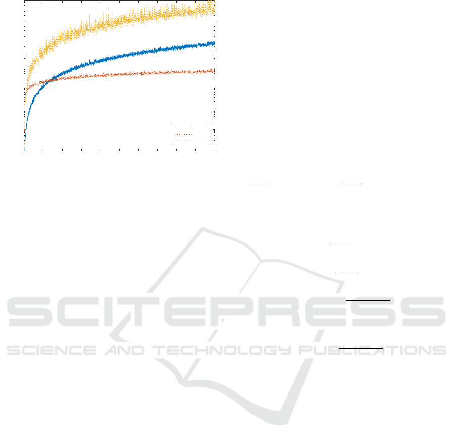
Figure 1: Dependency of MoNLs on growing variance P

for γ(x).

As a consequence of (35) the SIR algorithm pro-

vides a quantity for an estimation of the variance of

calculated SRs

var(SR(Q,ρ)) ≈ N · V

. (38)

4.2 Relation of Square Error of

Estimated Integral with MoNL

The variance of the calculated SRs, var(SR(Q,ρ))

approximately given by N · V

, can be viewed as a

measure of nonlinearity, because it is zero for a lin-

ear function and there is a reason to believe that for

a growing strength of nonlinearity of γ, the variance

grows as well. The quantity N · V

will be denoted

as MoNL

SIR

. An illustration follows to support this

belief.

To facilitate analyzing of behavior of MoNL

SIR

for different nonlinearities, the following approach

will be adopted: Instead of changing the function γ

for a ﬁxed

x and P

, the nonlinear function γ will be

ﬁxed and the variance P

will change. The variance

governs the region over which the nonlinearity is

analyzed and hence for growing P

, i.e., enlarging

the region, the nonlinearity should become stronger.

The following static example has been chosen:

Assume the function of interest y = γ(x) = x

, the ran-

dom variable x is given by mean value ¯x = 0.1 and

variance P

∈ (0, 2). The SIR was used to calcu-

late MoNL

SIR

with the parameter N

max

= 100. The

MoNL

DGM

and MoNL

WLS

used the same ζ-points to

calculate the value of the measure. In case of the

MoNL

WLS

, the weighting matrix was chosen as the

eye matrix. The Figure 1 depicts the results of the ex-

periment. All three measures inform the user of rising

inﬂuence of nonlinearity for growing variance P

4.3 Prediction of Number of Iterations

in SIR

In some cases, the user may specify the stopping con-

dition in Algorithm 2 by the error tolerance ε only,

i.e., without speciﬁcation of the maximum number of

iterations N

max

. Throughout the iterations, it is possi-

ble to predict the number of steps required to achieve

all elements of V

to be lower than ε

. The proce-

dure is as follows: At each iteration N the variance

var(SR(Q,ρ)) can be estimated by N · V

. Consider

TOT

being a number of iterations such that after N

TOT

steps the variance V

TOT

error will be approx-

imately

TOT

var(SR(Q,ρ)) ≈

TOT

· N · V

TOT

(39)

and the maximum element of

TOT

will be smaller

than ε

, i.e., max(

TOT

) < ε

. Hence

max

TOT

= max



TOT

· N · V



< ε

TOT

maxV

< ε

N · max V

< N

TOT

. (40)

Thus the total number of steps can be estimated by

TOT



N · max V



, (41)

where d·e is the ceil function rounding to the nearest

larger integer.

The total number of steps N

TOT

gives the user the

information about how long it will take to obtain the

integral value

with the desired accuracy ε.

5 MSE ESTIMATED BY SIF

In this section the SIF will be analyzed in the terms of

the MSE and based on the ﬁndings from the previous

section and calculation of the MSE estimate will be

proposed.

5.1 Theoretical values of MSE

The GFs compute the CM P

k|k

, which can be seen as

an estimate of the MSE, i.e.,

k|k

≈ MSE = E



−

k|k

)(·)



. (42)

Now, the true MSE will be calculated and compared

with the CM

k|k

calculated by the SIF.

ICINCO 2016 - 13th International Conference on Informatics in Control, Automation and Robotics

358

For convenience, consider the estimate

k|k

(10) as

an afﬁne function of z

, i.e.,

k|k

= Az

+ b, (43)

where

A =

(

)

−1

, (44)

b =

x − A

z. (45)

Note that for clarity purposes the subscript k|k −1 will

be omitted for the predictive moments.

Substituting (43) into (42) yields



−

k|k

)(·)



= E[(x

− Az

− b)(·)

]

{z }

E[αα

]

= E



−

x − A(z

−

z))(·)



| {z }

E[(α−

α)(α−

α)

]

x − A

z − b][·]

| {z }

(46)

After applying the expectation operator the MSE is



−

k|k

)(·)



= P

−P

| {z }

−AP

| {z }

+ AP

| {z }

x − A

z − b][·]

| {z }

, (47)

where the estimator-related expressions were labeled

as A,B,C, and D. In the following paragraphs these

expressions will be analyzed separately by substitut-

ing (44) and (45) into the terms:

A = −P

= −P

(

)

−1

= −(

)(

)

−1

= −

(

)

−1

−

) −

(

)

−1

(

)

−1

−

(

)

−1

−

(

)

−1

(48)

B = A

(49)

C = AP

(

)

−1

(

)(

)

−1

(

)

−1

(

)

−1

(

)

−1

(50)

D = (

x − A

z − b)(·)

= (A

z − A

z)(A

z − A

(

)

−1

(

)

−1

. (51)

Hence, (47) can be rewritten as



−

k|k

)(·)



= P

+ A + B + C + D

= P

−

(

)

−1

| {z }

k|k

(

)

−1

| {z }

−

(

)

−1

− P

(

)

−1

| {z }

(

)

−1

(

)

−1

| {z }

(

)

−1

(

)

−1

| {z }

k|k

+ 2E + F +G + H

| {z }

MSE

err

k|k

, (52)

which can be understood as the sum of the SIF esti-

mate

k|k

of P

k|k

and a sum of numerical integration

caused error terms 2E, F , G and H (denoted as the

MSE

err

k|k

), which provides the error in approximation

of the MSE. By using the estimate V

of the integral

mean squared error related to calculation of

and

, which will be denoted as V

, V

and V

respectively, the terms E, F , G and H of MSE

err

k|k

can

be estimated as:

The term E can be calculated during computation of

using (36) as

(

)

−1

≈

N − 1

∑

i=1



SR(Q

,ρ

) −



(

)

−1



SR(Q

,ρ

) −



, (53)

where the SR approximate P

at i-th iteration.

The term F depends on the true CM P

. Thus the

expectation of F w.r.t. the Q and ρ used for

computation is zero, i.e.,

E[F ] = E



−

(

)

−1

−P

(

)

−1



=0.

(54)

The term G can be approximated after applying the

expectation operator due to mutual independence

and

z. Then, E[

] is the variance of

z, which can be approximated by V

, i.e.,

G ≈

(

)

−1

(

)

−1

. (55)

The term H cannot be replaced by its estimate as

and

are clearly dependent. Here, the ap-

proach replacing

by its interval estimate will

On Nonlinearity Measuring Aspects of Stochastic Integration Filter

359

0.5

0.90.80.7

MSE

0.60.50.40.30.20.10

0.4

0.3

0.1

0.2

0.5

histogram of 3-σ bounds

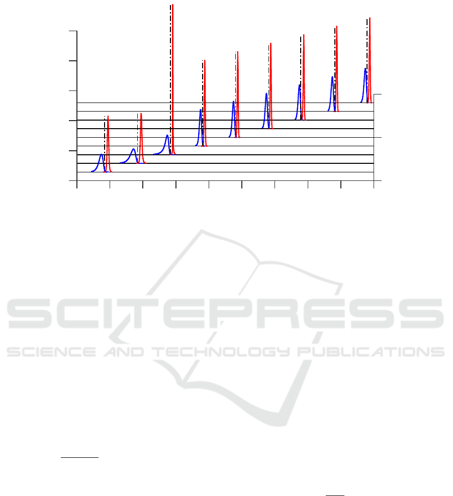
Figure 2: MSE interval estimates (blue solid line - low limit histogram, red solid line - high limit histogram) and true MSE

(black vertical dashed line) for several values of covariance P

be adopted. As

has multivariate Gaussian dis-

tribution with zero mean and matrix of variances

given by V

in H can be replaced by a ma-

trix where its each element is a 3-σ interval es-

timate of the corresponding element of

. This

matrix of 3-σ interval estimates will be denoted as

. Then the term H can be approximated as

H ≈

(

)

−1

(

)

−1

. (56)

Hence, the true MSE can be estimated by a 3-σ inter-

val estimate taking into account all errors of numeri-

cal integration being neglected so far. This interval is

given by substituting estimates (53) - (56) into (52),

i.e.,



−

k|k

)(·)



k|k

+ MSE

err

k|k

≈

k|k

N(N − 1)

∑

i=1



SR(Q

,ρ

) −

(γ)



× (

)

−1



SR(Q

,ρ

) −

(γ)



(

)

−1

(

)

−1

(

)

−1

(

)

−1

. (57)

The relation (57) represents the improved estimate of

the MSE provided by the SIF. This improvement is

facilitated by the SIR, which in addition to the ap-

proximate integration also calculates the MSE of the

calculation error V

. This quantity is not provided by

any other GF.

5.2 Example

In the following example MSE

err

k|k

from the previous

section is illustrated. Again the same static scalar ex-

ample as in Section 4.2 has been chosen, i.e.,

= x

+ v

, (58)

where v

∼ N (0, R) is the measurement noise with

zero mean Gaussian distribution and its variance is

R = 10

−4

, the random variable x

is Gaussian with

∼ N (x

;0.1, P

), where P

had been tested for

values 0.1,0.2, . .. , 0.9. The test scenario was per-

formed in the scope of N

= 10

independent Monte

Carlo simulations of state x

estimation. The ﬁlter-

ing estimate ¯x

0|0

and most importantly the ﬁltering

CM P

0|0

were obtained using the SIF with parame-

ters N

max

= 100 and ε = 10

−4

. The relatively high

simulation count secured high precision computation

of the true MSE value denoted as

MSE

true

∑

i=1

( ¯x

0|0

− x

)

, (59)

where superscript i denotes i-th Monte Carlo simula-

tion, x

is the true state at the i-th simulation and ¯x

0|0

is its ﬁltering estimate. The MSE

true

was compared to

the MSE estimate (57) calculated by the SIF.

The results are depicted in Figure 2, where his-

tograms of low (blue) and high (red) limits of the 3-σ

intervals are plotted. The true values of the MSE are

depicted as dashed vertical lines. The results conﬁrm

for several values of P

, that the SIF is capable to pro-

vide quality interval estimate of the MSE. The SIF is

ICINCO 2016 - 13th International Conference on Informatics in Control, Automation and Robotics

360

thus very versatile estimator capable of high quality

self-assessment

6 CONCLUSIONS

The paper dealt with the Bayesian state estimation of

nonlinear stochastic dynamic systems and speciﬁcally

with the stochastic integration ﬁlter, which is based

on a stochastic integration rule. Within the iterative

algorithm of the SIF an instrument for measuring the

nonlinearity was discovered. The instrument uses a

quantity, which is a byproduct of the SIR, which has

been used in the stopping condition so far. Such in-

formation provides an information of how much the

nonlinearity in the system violates the Gaussian as-

sumption of the SIF. The paper also provided a re-

lation that can be used to predict the number of SIR

iterations required to achieve the accuracy requested

by the user.

Further, in the paper a method to calculate im-

proved estimates of the MSE was developed. It was

shown that the MSE contains additional terms besides

the conditional variance matrix provided by the stan-

dard GFs. By utilizing the SIR byproducts the addi-

tional terms can be estimated by interval estimate. By

including the additional term estimates the SIF is able

to provide more accurate information about its state

estimates. Both the new nonlinearity measure and the

improved MSE were illustrated using simple numeri-

cal examples.

The interesting part of the discoveries made in this

paper is that it opens wide area for a future work. The

SIF can be further improved in terms of saving com-

putational demands, when the measurement function

is almost linear, or when the function is strongly non-

linear an execution of the algorithm can be paused and

for example Gaussian sum approach can be adopted

to improve estimate quality.

ACKNOWLEDGEMENTS

This work was supported by the Czech Science Foun-

dation, project no. GA 16-19999J.

REFERENCES

Arasaratnam, I. and Haykin, S. (2009). Cubature Kalman

ﬁlters. IEEE Transactions on Automatic Control,

54(6):1254–1269.

Arasaratnam, I., Haykin, S., and Elliott, R. J. (2007).

Discrete-time nonlinear ﬁltering algorithms using

Gauss–Hermite quadrature. Proceedings of the IEEE,

95(5):953–977.

Bates, D. M. and Watts, D. G. (1988). Nonlinear Regression

Analysis and Its Applications. John Wiley & Sons.

Doucet, A., De Freitas, N., and Gordon, N. (2001). Se-

quential Monte Carlo Methods in Practice, chapter

An Introduction to Sequential Monte Carlo Methods.

Springer. (Ed. Doucet A., de Freitas N., and Gordon

N.).

Dun

ık, J., Straka, O., and

Simandl, M. (2013a). Nonlinear-

ity and non-Gaussianity measures for stochastic dy-

namic systems. In Proceedings of the 16th Interna-

tional Conference on Information Fusion, Istanbul.

Dun

ık, J., Straka, O., and

Simandl, M. (2013b). Stochas-

tic integration ﬁlter. IEEE Transactions on Automatic

Control, 58(6):1561–1566.

Genz, A. and Monahan, J. (1998). Stochastic integration

rules for inﬁnite regions. SIAM Journal on Scientiﬁc

Computing, 19(2):426–439.

Ito, K. and Xiong, K. (2000). Gaussian ﬁlters for nonlinear

ﬁltering problems. IEEE Transactions on Automatic

Control, 45(5):910–927.

Julier, S. J. and Uhlmann, J. K. (2004). Unscented ﬁltering

and nonlinear estimation. IEEE Review, 92(3):401–

421.

Kramer, S. C. and Sorenson, H. W. (1988). Recursive

Bayesian estimation using piece-wise constant ap-

proximations. Automatica, 24(6):789–801.

Li, X. R. (2012). Measure of nonlinearity for stochastic sys-

tems. In Proceedings of the 15th International Con-

ference on Information Fusion, Singapore.

Mallick, M. (2004). Differential geometry measures of non-

linearity with applications to ground target tracking.

In Proceedings of the 7th International Conference on

Information Fusion, Stockholm, Sweden.

Nørgaard, M., Poulsen, N. K., and Ravn, O. (2000). New

developments in state estimation for nonlinear sys-

tems. Automatica, 36(11):1627–1638.

Ristic, B., Arulampalam, S., and Gordon, N. (2004). Be-

yond the Kalman Filter: Particle Filters for Tracking

Applications. Artech House.

Sorenson, H. W. (1974). On the development of practical

nonlinear ﬁlters. Information Sciences, 7:230–270.

On Nonlinearity Measuring Aspects of Stochastic Integration Filter

361