
A Robust Approach for Improving the Accuracy of IMU based Indoor
Mobile Robot Localization
Suriya D. Murthy, Srivenkata Krishnan S, Sundarrajan G,
Kiran Kassyap S, Ragul Bhagwanth and Vidhya Balasubramanian
Department of Computer Science and Engineering, Amrita School of Engineering,
Amrita Vishwa Vidyapeetham, Amrita University, Coimbatore, India
Keywords:
Robot Localization, Indoor Localization, Sensor Fusion, Inertial Sensors, Dead Reckoning.
Abstract:
Indoor localization is a vital part of autonomous robots. Obtaining accurate indoor localization is difficult in
challenging indoor environments where external infrastructures are unreliable and maps keep changing. In
such cases the robot should be able to localize using their on board sensors. IMU sensors are most suitable
due to their cost effectiveness. We propose a novel approach that aims to improve the accuracy of IMU based
robotic localization by analyzing the performance of gyroscope and encoders under different scenarios, and
integrating them by exploiting their advantages. In addition the angle computed by robots to avoid obstacles
as they navigate, is used as an additional source of orientation estimate and appropriately integrated using a
complementary filter. Our experiments that evaluated the robot over different trajectories demonstrated that
our approach improves the accuracy of localization over applicable existing techniques.
1 INTRODUCTION
Robotic indoor localization is a method in which the
position and orientation of the mobile robot is deter-
mined with respect to the indoor environment and is
an important part of any autonomous mobile robot.
Autonomous robot systems are commonly being used
during disaster response, in industries, as assistive
robots etc. In order to support the effective func-
tioning of robots in such scenarios there is a need for
accurate and efficient indoor localization, navigation
and mapping methods. One of the fundamental chal-
lenges in indoor environments is localization and this
supports the other two functionalities. In this paper
our primary goal is accurate self localization of mo-
bile robots in indoor environments.
Several approaches have been designed for mo-
bile robot localization, which include infrastructure
and non-infrastructure based methods. Infrastructure
based approaches use existing WiFi or RFID installa-
tions to help localize the robot (Choi et al., 2011; Li,
2012; Zhang et al., 2014). However, the accuracy of
these approaches are environment dependent, there-
fore we need solutions that do not rely on external
infrastructure. Approaches that do not rely on infras-
This work has been funded in part by DST(India) grant
DyNo. 100/IFD/2764/2012-2013
tructure use laser range finders, on board cameras and
inertial sensors for localization of the robot (DeSouza
and Kak, 2002; Guran et al., 2014; Surmann et al.,
2003). Laser range finders have high accuracy, but
are expensive. Camera based approaches are effec-
tive in many situations, but are computationally com-
plex and perform poorly in low light conditions and
in presence of occlusions.
Cost effectiveness, practicality, and ease of use
has popularized the use of inertial sensors and digi-
tal encoders for localization purposes (Guran et al.,
2014), and are widely employed by dead reckon-
ing based approaches. While accelerometers and en-
coders have been used for distance estimates, gyro-
scopes and magnetometer sensors have been used to
estimate orientation. However the accuracy of these
sensors are affected due to accumulation of noise and
drift errors from accelerometers and gyroscopes re-
spectively. Digital encoders are affected by slippage
and other errors. To overcome these errors, map
matching techniques and sensor fusion techniques
have been proposed (Elmenreich, 2002; Xiao et al.,
2014).
In map matching, accuracy is improved by con-
sidering salient features in the map and reposition-
ing the robot based on it. Techniques like those de-
scribed in (Xiao et al., 2014) use probabilistic ap-
436
Murthy, S., S, S., G, S., S, K., Bhagwanth, R. and Balasubramanian, V.
A Robust Approach for Improving the Accuracy of IMU based Indoor Mobile Robot Localization.
DOI: 10.5220/0005986804360445
In Proceedings of the 13th International Conference on Informatics in Control, Automation and Robotics (ICINCO 2016) - Volume 2, pages 436-445
ISBN: 978-989-758-198-4
Copyright
c
2016 by SCITEPRESS – Science and Technology Publications, Lda. All rights reserved

proaches for map matching and thereby localization.
Sensor fusion techniques can be used to combine the
data from different sensors and improve their accu-
racy. Sensor fusion can be achieved by simple ag-
gregation based approaches or by applying filters like
Kalman, extended Kalman and Complementary fil-
ters (Kam et al., 1997). The current state of art in
Kalman filter based approaches use two or more dif-
ferent position and orientation estimates. The inputs
for the Kalman filter are from sensors embedded in
the robot and external features (landmarks, corridors,
walls etc.) present in the indoor environment where
the robot navigates. However accurate both sensor fu-
sion based and map matching based techniques may
be, they are ineffective when maps are incomplete and
the environment consists of dynamic obstacles. Ad-
ditionally they are computationally expensive. There-
fore a cost effective approach that does not completely
rely on a map is essential.
In this paper we propose an approach that effec-
tively combines the advantages of the encoders and
gyroscopes to improve the accuracy of localization of
the robot. While existing techniques like gyrodome-
try (Ibrahim Zunaidi and Matsui, 2006) have been de-
veloped, which use Kalman Filters for sensor fusion,
their performance is affected when accelerometers are
ineffective (as in the case of wheeled robots). Our
approach exploits the curvature of the robot’s trajec-
tory to determine when the gyroscopes and encoders
are used. This helps limit the continuous use of the
gyroscope thereby reducing drift errors. In addition
we exploit the obstacle avoidance capabilities of au-
tonomous robots to provide another source of orienta-
tion estimate. This is combined with the gyroscope’s
orientation estimate using complementary filter to im-
prove the localization accuracy.
The rest of the paper is organized as follows: Sec-
tion 2 outlines the state of art in robotic localization in
detail and positions our work with respect to it. Next
we discuss how the individual sensors are used for
distance and orientation estimate in Section 3 and ex-
plain our proposed approach in Section 4. Finally we
evaluate our approach for different scenarios (Section
5) and conclude in Section 6.
2 RELATED WORK
Many localization techniques have been developed
and implemented in robots over a period of time.
Common indoor localization methods for robots rely
on external infrastructures and sensors which are part
of the robot. Localization techniques that use RF
technologies such as RFID, WiFi and bluetooth (Choi
et al., 2011; Li, 2012; Zhang et al., 2014) rely on ad-
ditional external infrastructure such as RF antennas
and ultrasonic transceivers placed in the environment.
On the other hand, techniques that use cameras, laser
range finders or inertial sensors(DeSouza and Kak,
2002; Guran et al., 2014; Surmann et al., 2003) do
not rely on external infrastructure.
In the infrastructure based approaches, RF based
localization is one of the most prevalent techniques
and is easy to implement. In RF based methods,
the robot requires external infrastructure like anten-
nas/reference tags placed in the environment for com-
munication with the receiver carried by the robot.
RF based localization techniques can either use fin-
gerprinting or non-fingerprinting approaches. The
non-finger printing approaches include trilateration
method and angulation techniques(AOA) (Liu et al.,
2007). The trilateration method estimates the posi-
tion of the target with respect to the reference points
using the Received Signal Strength Indication (RSSI)
values (Easton and Cameron, 2006; Granados-Cruz
et al., 2014). This method fails to locate mobile node
in multipath dense environment. The WiFi finger-
printing technique compares the RSSI observations
made by the mobile node with a trained database
to determine the location of the moving object (Li,
2012). Deterministic approaches such as k-Nearest
Neighbors(k-NN) (Kelley, 2015), decision tree meth-
ods (Erinc, 2013) and probabilistic methods that in-
clude Bayesian, Hidden Markov Model (HMM) have
been used in fingerprinting approach. In RFID based
localization, a large number of RFID tags placed in
the environment act as reference points. Hence, when
a new RFID tag enters the space, the signal strength
is compared with the reference points’ signal strength
and location of the robot is determined (Choi et al.,
2011; Zhang et al., 2014). In both RFID and WiFi fin-
ger printing approaches, the collection of data set (of-
fline phase) is tedious and time consuming. It also re-
quires frequent updation of fingerprint maps and spe-
cial approaches are needed to reduce the cost of up-
dation (Krishnan et al., 2014).
The techniques that do not rely on infrastructure
involve the use of LIDAR (Light Detection and Rang-
ing), cameras and inertial sensors. Camera based ap-
proaches use the entire visual information or interest
points or combination of all these as input in deter-
mining the location of the robot(DeSouza and Kak,
2002). These methods are usually prone to errors due
to occlusions, changes in scale, rotation and illumina-
tion. In LIDAR based approaches, lasers have been
used to emit pulses that are reflected off a rotating
mirror from which time of flight is determined and
used to calculate distances(Surmann et al., 2003). The
A Robust Approach for Improving the Accuracy of IMU based Indoor Mobile Robot Localization
437
main drawback here is that the laser range finders are
expensive.
Inexpensive sensors such as accelerometers, gy-
roscopes and encoders are increasingly being used
in localization. These IMU sensors are commonly
used in dead reckoning, where new state estimates are
calculated with the help of prior states(Ahn and Yu,
2007). Accelerometers and encoders have been used
to find the distance while gyroscope and magnetome-
ter sensors have been used to determine the orienta-
tion (Guran et al., 2014). These methods do not give
accurate results because accelerometer suffers from
noise error, gyroscope suffers from static drift and
magnetometers are error-prone in places where mag-
netic interferences are high, especially in indoor en-
vironments. The encoders suffers from either system-
atic(unequal wheel dimensions and kinematic imper-
fections) or non-systematic errors(wheel slippage and
irregularities of the floor) and can be removed to a cer-
tain extent using the UMBmark test(Borenstein and
Feng, 1994). To overcome the inefficiencies of these
sensors we need to effectively combine the data from
multiple sensors. Sensor fusion based approaches
have been proposed to achieve this. The sensor fu-
sion in this context is the translation of different sen-
sory inputs into reliable estimates(Elmenreich, 2002).
Filters like Kalman and complementary filters have
been widely used for sensor fusion thereby improv-
ing the accuracy to some extent (Kam et al., 1997).
Map matching based techniques have also been ap-
plied (Xiao et al., 2014) that improve the accuracy of
localization accuracy using probabilistic approaches.
As mentioned in previous section, the above methods
fail when the map is not reliable and environment is
dynamic.
Therefore we need a better method that is able to
effectively localize the robot with minimum overhead
and no external infrastructure. In addition it must be
able to exploit the advantage of different sensors to
improve accuracy and without relying on maps. In
this paper we aim to achieve this using a novel deci-
sion based approach that uses the scenarios where dif-
ferent sensors work accurately. The next sections will
describe our approach for improving the localization
accuracy of indoor robots using inertial measurement
units.
3 SYSTEM OVERVIEW
Before we describe our approach we first introduce
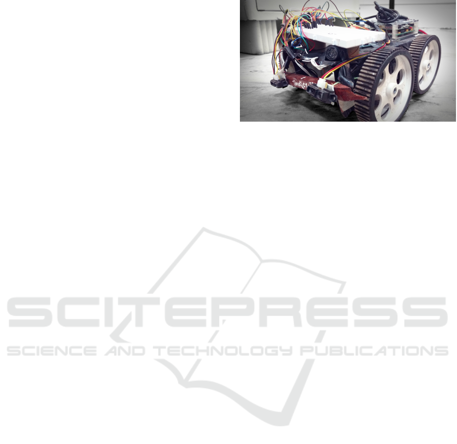
our robot, its system and its sensors. An image of our
robot is shown in Fig 1. Our robot is a four wheeled
autonomous light weight vehicle and has a dimension
Figure 1: Our 4-wheeled mobile robot.
of 105mm*55mm*57mm. Each of the 4 wheels has
a diameter of 110mm. The robot is equipped with
bStem (bst, 2015) single chip computer, an Arduino
micro controller, sensors and motor drivers. The en-
vironment in which the robot navigates is a partially
known environment, in which walls and corridors are
known but any furniture or moving obstacles are un-
known.
The robot is defined by its pose p which is given
at time t as,
p = [x
t
,y
t
,θ
t
]
where x
t
,y
t
represents the position estimate and θ
t
represents the orientation estimate.
To measure the distance travelled by the robot,
two quadrature encoders associated with the stepper
motors are added to the rear wheels of the robot. It
must be noted that this is a rear wheel driven differen-
tial driven robot and speed is controlled to avoid slips
and keep the kinematic center at the middle of the rear
wheels. These encoders output the left and right ticks
(l, r), using which the distance (dist) travelled by the
robot is calculated as dist = (l + r)/2. Since we do
not use accelerometers, this is the only source of dis-
tance estimate.
The encoders also provide us with an estimate of
the robot’s orientation θ
e
. The tri-axial gyroscope
present in bStem provides the angular rates with re-
spect to each axis. Using the z-axis angular rate we
calculate the orientation angle θ
g
. Two ultrasonic and
two infrared sensors are embedded on either sides in-
front of the robot. Both the sensors return the dis-
tance between the obstacle and robot. This data serves
to provide us with an additional orientation estimate.
We use the encoders to determine the distance esti-
mate and a combination of gyroscope, encoders and
obstacle avoidance sensors for orientation estimate to
effectively determine pose. The mathematical deter-
mination of position and orientation estimate from en-
coders, gyroscope and obstacle avoidance sensors are
explained below.
ICINCO 2016 - 13th International Conference on Informatics in Control, Automation and Robotics
438

3.1 Position and Orientation Estimation
using Encoders
The encoders provide ticks l and r from the left and
right motors respectively. The width of the robot is
defined as W . Using these, the position and orienta-
tion is calculated by applying geometric techniques
(Jensfelt, 2001). In this technique the pose is esti-
mated for the following two cases:
• Robot is taking turns.
• Robot is moving straight.
Case 1: Determination of Pose When the Robot is
Taking Turns
When the robot is taking turns, there is a difference
in the ticks between the right and left encoders. This
information is used to estimate the curvature of the
robots path (based on the previous position p
0
) and
hence determine the pose p. The heading direction
changes when the robot turns. The current orientation
is the heading angle which is based on the previous
orientation, and α. The new orientation estimate θ
e
(t)
is calculated as follows,
θ
e
(t) = θ
e
(t −1) + α (1)
Here the angle α represents the change in heading an-
gle of the robot during traversal from previous posi-
tion to the current position. The new position estimate
(x(t), y(t)) is determined as follows:
x(t) = C
x
+ (R + (W /2))sin(θ
e
(t)) (2)
y(t) = C
y
+ (R + (W /2))(− cos(θ
e
(t))) (3)
where C(C
x
,C
y
) is the center of the extended circle
where the arc traversed by the robot from previous
position to current position lies. Similarly, this can be
extended for the calculation of new pose when robot
turns right.
Case 2: Determination of Pose When the Bot is
Moving Straight
When the robot is moving straight, there is no change
in its orientation, and the left ticks are equal to the
value of right ticks. So, the new orientation estimate
is same as the orientation at time t − 1,
θ
e
(t) = θ
e
(t −1) (4)
Now, the corresponding pose x(t),y(t) is calculated as
given below,
x(t) = x(t − 1) + l(cos(θ
e
(t))) (5)
y(t) = y(t − 1) + l(sin(θ
e
(t))) (6)
3.2 Orientation Estimate using
Gyroscope
Gyroscope is a sensor used to measure angular veloc-
ity. In our robot, the L3GD20 MEMS motion sensor
3-axis digital gyroscope, which is part of the bStem
provides angular velocities along three axes x,y,z re-
spectively. The sensitivity of the gyroscope is set
at 250dps, ideal for a robotic system that undergoes
heavy vibrations due to motor and chassis movement.
The goal is to calculate the orientation angle of the
robot over a period of time, which is done by integrat-
ing the angular velocity about the z-axis over a certain
time interval. In order to get reliable angle estimates
we first calculate and eliminate the offset and noise of
our gyroscope and they are calculated as follows:
offset =
1
N
N
∑
i=0
ω (7)
where ω is the angular velocity at that instant of time
and N represents the number of angular velocity val-
ues taken.
noise = max(|ω
i
− offset|) 0 ≤ i ≤ N (8)
where ω
i
is the angular velocity at that instant. Noise
is calculated for all three axes. The angular velocities
which fall in the range of [−noise,noise] are ignored
and the remaining values are taken for the calculation
of orientation. The orientation angle θ
g
(t) at time t is
given by,
θ
g
(t) = θ
g
(t −1) + ω
i
dt (9)
where dt represents the time period over which ω
i
can
be periodically integrated to determine the angle, in
our case this value is equal to 20ms. Using the above
θ
g
(t) value we estimate the orientation and position.
The position estimate is calculated using previous po-
sition values, the newly calculated orientation value
and the distance estimate from encoders (dist) and is
determined as follows.
x(t) = x(t − 1) + dist ∗ cos(θ
g
(t)) (10)
y(t) = y(t − 1) + dist ∗ sin(θ
g
(t)) (11)
3.3 Orientation Estimate using Obstacle
Avoidance Sensors
In general orientation estimates come from the en-
coders, gyroscopes or magnetometers. Here we are
also using orientation estimates based on information
from obstacle avoidance sensors. Robots use obsta-
cle avoidance systems to avoid obstacles, and plan
their trajectory based on the distance between them
and the obstacle. At each point, while the obstacle is
A Robust Approach for Improving the Accuracy of IMU based Indoor Mobile Robot Localization
439

still in range, the autonomous robot calculate the cur-
vature angle required to safely maneuver itself. This
angle is only known when the obstacle is detected,
and it can be reasonably assumed that the robot’s ac-
tual trajectory during navigation is close to the esti-
mated trajectory determined for obstacle avoidance.
This estimated angle therefore is used by our algo-
rithm as an additional source of orientation estimate.
We explain the orientation estimation using the obsta-
cle avoidance system below.
In this paper we consider the ultrasonic and in-
frared sensors for obstacle avoidance. The sensor
specifications are given below,
1. Ultrasonic Range Finder XL-EZ3 (MB1230)
which has a range of 20cm to 760cm and a res-
olution of 1cm is used to detect obstacles present
in long range.
2. Sharp GP2Y0A41SK0F IR Distance Sensor
which has a range of 4cm to 30cm is used to de-
termine obstacles in close range.
A robot that is moving autonomously takes nav-
igational decisions based on the output from the
above sensors. An obstacle avoidance method
(Widodo Budiharto and Jazidie, 2011), is adapted to
calculate the orientation of the robot as explained be-
low. When an obstacle is detected, the two ultrasonic
sensors return the distances (d
lu
,d
ru
) between the ob-
stacle and corresponding left and right sensors on the
robot. d
sa f e
, the flank safety distance, is the mini-
mum distance at which robot can start to maneuver to
avoid obstacle. This value is calculated experimen-
tally based on the range of the ultrasonic sensors and
width of the robot. To determine the angle from the
distances given by ultrasonic and infrared sensors, the
following cases must be considered.
case 1: d
lu
> d
sa f e
and d
ru
> d
sa f e
When there
is no obstacle in front of the robot, it can continue
to move in the same direction. Hence the orientation
angle θ
oa
(t) at time t is same as the previous angle
θ
oa
(t −1).
case 2: d
lu
< d
sa f e
and d
ru
> d
sa f e
In this case the
robot has to take a right turn in order to avoid the ob-
stacle. The closer the robot is to the obstacle the wider
it has to turn and vice versa. The ideal angle, θ
oa
(t)
for the robot to avoid the obstacle is calculated using
the distance from left ultrasonic sensor as follows:
θ
oa
(t) = θ
oa
(t −1) −
π
2
(
k
θu
d
lu
) (12)
where k
θu
represents the collision angle constant for
the ultrasonic sensor, which is calculated based on
d
sa f e
and d
lu
.
case 3: d
lu
> d
sa f e
and d
ru
< d
sa f e
When the bot
has to turn left in order to avoid obstacle, the ideal
angle is calculated using the distance from the right
ultrasonic sensor and the angle is calculated similarly,
θ
oa
(t) = θ
oa
(t −1) +
π
2
(
k
θu
d
ru
) (13)
case 4: d
lu
< d
sa f e
and d
ru
< d
sa f e
When the robot
is too close to the obstacle, this case comes into pic-
ture. Here, we use the distances d
ri
, and d
li
returned
by the infrared sensors. The orientation is estimated
similarly. The angle calculation for right turn is given
by,
θ
oa
(t) = θ
oa
(t −1) − n ∗ (
π
2
)(
k
θi
d
ri
) (14)
Similarly, the angle calculation for left turn is given
by,
θ
oa
(t) = θ
oa
(t −1) + n ∗ (
π
2
)(
k
θi
d
li
) (15)
where n is experimentally calculated to increase or de-
crease the rotation appropriately to avoid close obsta-
cles. k
θi
is the collision angle constant for infrared
sensors.
Finally, if the robot is too close to the obstacle and
is impossible for it to maneuver an obstacle smoothly,
i.e. if d
lu
< d
n
, then the robot moves backwards by
a certain distance and checks for all the above pos-
sibilities and estimates the orientation angle. d
n
is
the maximum distance before which the robot should
start maneuvering to avoid the obstacle. This value
is calculated experimentally based on the range of the
infrared sensors and width of the robot. The region
{d
sa f e
- d
n
}, is the buffer region for smooth maneu-
vering. Using the above equations, we estimate the
orientation angle based on the data from the obstacle
avoidance sensors.
Now that we have estimated the pose using the
individual sensors, the goal of our system is to im-
prove the accuracy by appropriately combining the
data from all of them.
4 CURVATURE BASED DECISION
SYSTEM
This section describes our novel approach to improv-
ing the location accuracy by fusing information from
the different sensors appropriately. In robotic local-
ization inaccuracies in orientation measure affects the
position more when compared to inaccuracies in dis-
tance measure(Borenstein and Feng, 1994). For ex-
ample, a robot with 8 inch wheel base and slip of 1/2
inch in one of the wheels results in an error of approx-
imately 3.5 degrees in orientation. So it is important
to have a highly accurate value of the orientation mea-
sure when compared to that of a distance measure.
ICINCO 2016 - 13th International Conference on Informatics in Control, Automation and Robotics
440

Our method assumes that the distance(l,r) measured
using the encoders is reliable, since the systematic er-
rors can be easily removed using UMBenchmark and
non-systematic errors do not affect the distance esti-
mate much, as explained in the above example. The
orientation estimate from encoders however are not
reliable since they undergo huge non-systematic er-
rors due to sudden turns and heavy slippage. Slight
deviations in distance due to non-systematic errors
results in huge deviations in orientations. The gyro-
scopes are generally accurate in estimating orienta-
tion, and is preferred over encoders. However, over
longer durations the performance degrades due to the
accumulation of drift errors. Our approach enhances
the accuracy of orientation estimation by a) reducing
the period over which the gyroscope value accumu-
lates, so that drift errors are minimized and b) fus-
ing the orientation estimates from gyroscope with ori-
entation estimates obtained to avoid obstacles as dis-
cussed in Section 3.3.
Inorder to actualize the above, the trajectory in
which the robot travels is analyzed. We identify the
part of the trajectory that is almost linear, so that ori-
entation measure from encoders can be used reliably.
In the other parts of the trajectory the gyroscope is
employed. To improve the accuracy further, the gy-
roscope data is fused with the angle estimated at the
current position by the robot to avoid obstacles. The
main steps in our approach are as follows
1. Estimation of curvature of the robot’s trajectory
2. Using the trajectory to determine the appropriate
sensor to use
3. Enhance orientation estimation accuracy using
a complementary filter to fuse orientation from
above step and obstacle avoidance system
A decision based approach is preferred to a fusion
based approach for determining the sensor to use
based on the curvature of the trajectory. Since it is
clear which sensors used perform better in different
scenarios we employ this approach.
4.1 Curvature Estimation
The robot’s trajectory is a 2D smooth plane curve.
The curvature of the past trajectory of the robot deter-
mines the sensor(s) to be used for the orientation esti-
mation at the current point. In order to find the curva-
ture, we find the angle between the slopes of tangents
drawn to the previous points P1(x,y) and P2(x,y) on
the trajectory. To draw the tangents we find the center
of curvature C(C
x
,C
y
) of the curve. We then calculate
the angle between the slopes of the tangents, which
Figure 2: Determination of slope.
gives the curvature at the point. This method is effi-
cient in curvature estimation since we only store the
previous two points of the trajectory and not the com-
plete trajectory to decide on the appropriate sensors.
To find the slope m1 of the tangent vector T at
point P1, we first find the slope n1 of the normal vec-
tor N at P1 passing through center of curvature C. The
slope of n1 is calculated using
n1 = (C
y
− P2(y))/(C
x
− P1(x)) (16)
The slopes m1 of the tangent vector T , which is
perpendicular to N is then calculated as the negative
of the inverse of n1; m1 = −1/n1. Similarly we cal-
culate m2, which is the slope of the tangent vector at
point P2.
Once these two slopes are calculated the degree of
curvature D
c
can be determined as follows
D
c
= tan
−1
((m1 − m2)/(1 + m1 ∗ m2)) (17)
This D
c
value helps us determine if the robot is trav-
elling in a near linear trajectory or on a curved path.
Using this we determine when to start aggregating the
gyroscope values and when to only rely on encoders.
A gyroscope controller is implemented to appropri-
ately switch between the encoders and gyroscope.
4.2 Gyroscope Controller
The gyroscope controller starts accumulating the gy-
roscope readings, and switches completely to the en-
coder based on start and stop threshold values. The
start threshold value µ1 is calculated by computing
the average of the degrees of curvature when the robot
begins to make a turn. When the robot completes a
maneuver by avoiding an obstacle and starts to follow
a linear trajectory, the average of degree of curvatures
of multiple linear paths is computed and used as the
stop threshold value µ2.
When the D
c
keeps increasing and goes over start
threshold value µ1, we initiate the gyroscope and use
it for orientation measure and allow it to summate as
the robot traverses the curved path. The accumulation
A Robust Approach for Improving the Accuracy of IMU based Indoor Mobile Robot Localization
441
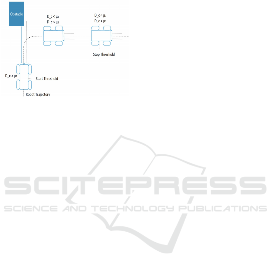
Figure 3: Determination of start and stop threshold.
of gyroscope values is stopped when the degree of
curvature becomes closer to the stop threshold value
µ2. Figure 3 shows this scenario. By doing this we
ensure that the gyroscope is not made to accumulate
continuously for a long time, thereby ensuring that
the drift errors from the gyroscopes are not a major
source of localization errors. When D
c
keeps decreas-
ing and becomes equal to or less than µ2, the encoders
are used for orientation estimation of the robot. Us-
ing the encoders when the D
c
is less than or equal to
the µ2, reduces the effect of the non systematic errors
resulting in an accurate position calculation. In order
to achieve the above the following conditions have to
be met,
1. µ2<<µ1, ensuring the left and right ticks are
equal in straight paths.
2. µ1 is given higher precedence than µ2, ensuring
gyroscope is started as soon as the robot begins to
make a turn.
In order to further increase the orientation estimate
obtained from gyroscope, it is fused with the an-
gle obtained from the obstacle avoidance sensors ex-
plained below.
4.3 Gyro-obstacle Fusion
To improve the accuracy of orientation estimates dur-
ing turns, the gyroscope values are fused with the
ideal angle estimated to avoid obstacles as explained
in Section 3.3. As discussed earlier it is our hypoth-
esis that robots tend to closely follow the trajectory
estimated to avoid obstacles. However the actual an-
gle taken by the robot to avoid the obstacle is not
controllable and hence is only known by the gyro-
scope. Therefore this estimated angle is fused with
the gyroscope angle to potentially enhance the accu-
racy. We use a complementary filter for this fusion
process since it is very easy and light to implement
making it perfect for embedded systems application
as in our case. The complementary filter is given by
the equation,
θ = αθ
g
+ (1 − α)θ
oa
(18)
where θ
g
is the angle obtained from gyroscope, θ
oa
is
angle obtained from obstacle avoidance sensors and α
is the factor which is determined experimentally.
Therefore, we get a good orientation estimate
from encoders, gyroscope and obstacle avoidance
system. This orientation is then combined with the
distance measure(l,r) from encoders to get the pose
estimate. On fusing the data by considering the ad-
vantages of individual sensors, the position is ob-
tained.
5 EXPERIMENTAL RESULTS
The previous sections discussed our approach for im-
proving the accuracy of localization by combining
data from different sensors used in our robot. In this
section we analyze the performance of this approach.
First we discuss the arena and experimental setup fol-
lowed by the metrics used for analyzing our algo-
rithm. We also discuss the methodology for obtaining
the ground truth.
The experiments are carried out in an arena of
dimensions 1710 ∗ 480cm
2
using a four wheeled au-
tonomous robot as shown in Figure 1. The arena is
then transformed into a grid of squares, each of area
900cm
2
. Obstacles are placed in different parts of the
arena. Different trajectories are considered for evalu-
ating our algorithm. In order to generate the ground
truth the grid is used to identify the points the robot
passed through. These points are plotted on a raster
map. The following algorithms are evaluated (it must
be noted that in all the techniques encoders provide
the distance estimate, and these techniques are used
for angle estimation)
1. Encoder based approach
2. Gyroscope based approach
3. Curvature based Decision Approach without in-
tegrating obstacle avoidance information (CDA-
nO)
4. Curvature based Decision Approach that uses all
three sensors (CDA-O)
To evaluate the performance of these approaches in
comparison to the ground truth we use the metrics as
discussed next.
ICINCO 2016 - 13th International Conference on Informatics in Control, Automation and Robotics
442
5.1 Metrics of Evaluation
The most important indicator in evaluating the per-
formance of a localization algorithm is accuracy. Ac-
curacy refers to how close the estimated trajectory as
obtained from the localization method is to the ground
truth. In order to determine the closeness, mean and
standard deviation of the Euclidean distance between
the ground truth and estimated point is calculated.
The mean Euclidean distance is the sum of Euclidean
distance at each corresponding point divided by the
total number of such corresponding points.
µ =
∑
N
i=0
(
p
((x
gt
− x
est
)
2
+ (y
gt
− y
est
)
2
))
N
(19)
(x
gt
,y
gt
) refers to the ground truth and (x
est
,y
est
) is
the estimated position from the localization method
used. While the mean provides the error estimates, the
standard deviation gives an idea of how consistently
the algorithm performs.
5.2 Performance Analysis
We evaluate the above mentioned approaches over the
arena specified. The evaluation is done by making the
robot navigate along different trajectories in the arena.
We have considered three trajectories and their corre-
sponding ground truth is plotted and used for compar-
ison. Table 1 shows the mean and standard deviation
of the euclidean distance error in the corresponding
trajectories and methods used for comparison respec-
tively.
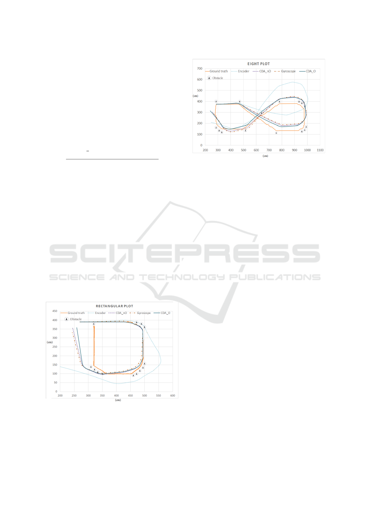
Figure 4: Performance for a Rectangular Trajectory.
5.2.1 Case 1: Rectangular Trajectory
The first case is when the robot traversed along the pe-
riphery of the arena resulting in a rectangular trajec-
Figure 5: Performance for an Eight Shaped Trajectory.
tory. Figure 4 shows the plot of the estimated trajec-
tories for different techniques along with the ground
truth trajectory. From the figure and the table we can
see that the average error of encoder based localiza-
tion is comparatively high. This is because, in the tra-
jectory, the robot has taken sharp turns, which leads
to slips and it affects the performance of the encoder
based method. The performance of gyroscope based
localization is better than encoder because its orienta-
tion estimates are more accurate during turns, and that
dictates the accuracy of the trajectory. The curvature
based approach improves the accuracy of the localiza-
tion over the gyroscope on average. However using
the orientation estimates from the obstacle avoidance
system further improves the accuracy. This supports
our hypothesis that the robot traverses nearly close
to the estimated trajectory needed to avoid obstacles.
Additionally since the gyroscope is the only measure
of the actual angle taken by the robot in this scenario,
fusing with the estimated angles helps the estimated
trajectory come closer to the ground truth. This leads
us to the conclusion that orientation estimates during
obstacle avoidance has high accuracies and can be re-
liably used.
5.2.2 Case 2: Eight Shaped Trajectory
Figure 5 shows the output of the different localization
methods when the robot is allowed to navigate in an
eight shaped trajectory. Here we can notice that since
there are not many sharp turns, the encoder perfor-
mance improves. Here too our curvature based ap-
proaches (both with and without input from obstacle
avoidance sensors) perform the best. While the gy-
roscope plays a major role in the improvement of ac-
curacy, the nature of the trajectory limits the curva-
ture based decision approach. However we can see
that employing the input from obstacle avoidance im-
A Robust Approach for Improving the Accuracy of IMU based Indoor Mobile Robot Localization
443
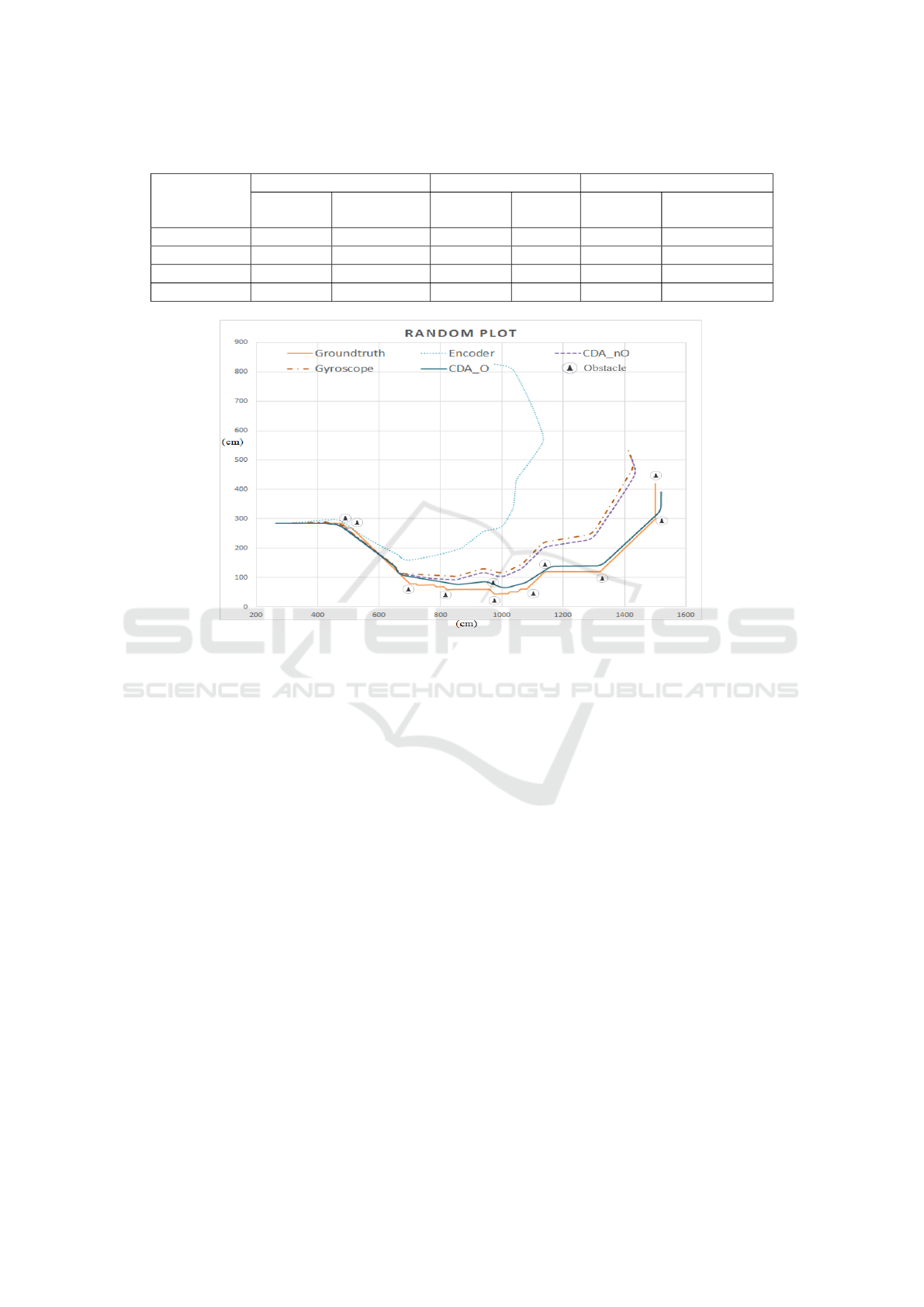
Table 1: Performance analysis of different techniques for different trajectories.
Methods
implemented
Trajectory 1(Rectangular) Trajectory 2(Eight) Trajectory 3 (Random Path)
Avg Error
(cm)
Std Dev
(cm)
Avg Error
(cm)
Std Dev
(cm)
Avg Error
(cm)
Std Dev
(cm)
Encoders 121.96 79.64 89.27 51.74 333.65 191.74
Gyroscope 40.50 22.49 44.22 26.86 75.33 44.26
CDA-nO 28.64 15.96 39.50 24.91 65.38 38.96
CDA-O 20.25 12.59 34.68 24.66 20.49 12.67
Figure 6: Random plot.
proves the accuracy to a certain extent.
5.2.3 Case 3: Random Trajectory
To obtain a better idea of how well our approach for
localization works, we allowed the robot to take a
random path filled with obstacles, and this path was
much longer than the previous ones. When the path
is longer, the drift errors in the gyroscope play a role.
Figure 6 shows the plots of the estimated trajectories
for this path. We can see that here that our curva-
ture based approach that utilizes the obstacle avoid-
ance system performs exceedingly well in compari-
son to all other strategies. This is because the path
has lot of obstacles and that is well exploited here.
The gyroscope performs poorest here, since it is more
prone to drift errors here. Therefore using the curva-
ture based approach helps reduce the drift error, and
improve accuracy to a small extent. While the ’o f f set
and ’noise’ is calibrated at the beginning, we propose
to update it at regular intervals, specially when the
robot is moving straight. Overall we can see that our
approach performs consistently well in all scenarios
and gives an accuracy of around 20 to 30 cm. We
also observe that considering the curvature and fus-
ing the estimate of the orientation from the obstacle
avoidance systems with gyroscopes significantly im-
proves accuracy. The trajectories generated by our ap-
proach are very close to the trajectory both in terms
of distance and the overall pattern, as can be seen in
the plots. The standard deviation values, specially for
the rectangular and random plots show that our ap-
proach not only provides good accuracies, but does
it consistently along the path. Additionally the over-
head of this approach is low and hence is easily im-
plementable in any autonomous robot.
6 CONCLUSIONS AND FUTURE
RESEARCH
In this paper we have described out approach for im-
proving the localization accuracy of indoor mobile
robots, which use inertial sensors for localization.
The curvature of the robot’s trajectory is analyzed to
determine when the gyroscope and encoder data are
to be used. In addition to improve the accuracy, ori-
entation estimates from obstacle avoidance systems
are fused with the gyroscope’s orientation estimates.
ICINCO 2016 - 13th International Conference on Informatics in Control, Automation and Robotics
444

Our experiments have shown that by using only gy-
roscopes as and when needed, and employing the ad-
ditional data from obstacle avoidance sensors, the lo-
cation accuracy is improved significantly. It is seen
that since environments usually have obstacles, and
robots have to navigate around them, using that as
a parameter is an effective approach for localization.
Our approach provides good accuracies at a low over-
head. However when the turns are very sharp, and
acute, our approach suffers. While our approach ac-
counts for gyroscope drift errors, more work needs to
be done to reduce it further for longer distances.
REFERENCES
(2015). bstem developer kit & integrated robotics platform:
www.braincorporation.com.
Ahn, H.-S. and Yu, W. (2007). Indoor mobile robot and
pedestrian localization techniques. In Control, Au-
tomation and Systems, 2007. ICCAS’07. International
Conference on, pages 2350–2354. IEEE.
Borenstein, J. and Feng, L. (1994). Umbmark: a method for
measuring, comparing, and correcting dead-reckoning
errors in mobile robots.
Choi, B.-S., Lee, J.-W., Lee, J.-J., and Park, K.-T. (2011). A
hierarchical algorithm for indoor mobile robot local-
ization using rfid sensor fusion. Industrial Electronics,
IEEE Transactions on, 58(6):2226–2235.
DeSouza, G. N. and Kak, A. C. (2002). Vision for mobile
robot navigation: A survey. Pattern Analysis and Ma-
chine Intelligence, IEEE Transactions on, 24(2):237–
267.
Easton, A. and Cameron, S. (2006). A gaussian error model
for triangulation-based pose estimation using noisy
landmarks. In Robotics, Automation and Mechatron-
ics, 2006 IEEE Conference on, pages 1–6. IEEE.
Elmenreich, W. (2002). Sensor fusion in time-triggered sys-
tems.
Erinc, G. (2013). Appearance-based navigation, localiza-
tion, mapping, and map merging for heterogeneous
teams of robots.
Granados-Cruz, M., Pomarico-Franquiz, J., Shmaliy, Y. S.,
and Morales-Mendoza, L. J. (2014). Triangulation-
based indoor robot localization using extended
fir/kalman filtering. In Electrical Engineering, Com-
puting Science and Automatic Control (CCE), 2014
11th International Conference on, pages 1–5. IEEE.
Guran, M., Fico, T., Chovancova, A., Duchon, F., Hubinsky,
P., and Dubravsky, J. (2014). Localization of irobot
create using inertial measuring unit. In Robotics in
Alpe-Adria-Danube Region (RAAD), 2014 23rd Inter-
national Conference on, pages 1–7. IEEE.
Ibrahim Zunaidi, Norihiko Kato, Y. N. and Matsui, H.
(2006). Positioning system for 4wheel mobile robot:
Encoder, gyro and accelerometer data fusion with er-
ror model method. In CMU Journal, volume 5.
Jensfelt, P. (2001). Approaches to mobile robot localization
in indoor environments. PhD thesis, RoyalInstitute of
Technology, Stockholm, Sweden.
Kam, M., Zhu, X., and Kalata, P. (1997). Sensor fusion
for mobile robot navigation. Proceedings of the IEEE,
85(1):108–119.
Kelley, K. J. (2015). Wi-fi location determination for se-
mantic locations. The Hilltop Review, 7(1):9.
Krishnan, P., Krishnakumar, S., Seshadri, R., and Bala-
subramanian, V. (2014). A robust environment adap-
tive fingerprint based indoor localization system. In
In Proceedings of the 13th International Conference
on Ad Hoc Networks and Wireless (ADHOC-NOW-
2014), volume 8487, pages 360–373.
Li, J. (2012). Characterization of wlan location fingerprint-
ing systems. Master’s thesis, School of Informatics,
University of Edinburgh.
Liu, H., Darabi, H., Banerjee, P., and Liu, J. (2007). Sur-
vey of wireless indoor positioning techniques and
systems. Systems, Man, and Cybernetics, Part C:
Applications and Reviews, IEEE Transactions on,
37(6):1067–1080.
Surmann, H., N
¨
uchter, A., and Hertzberg, J. (2003). An au-
tonomous mobile robot with a 3d laser range finder for
3d exploration and digitalization of indoor environ-
ments. Robotics and Autonomous Systems, 45(3):181–
198.
Widodo Budiharto, D. P. and Jazidie, A. (2011). A robust
obstacle avoidance for service robot using bayesian
approach. International Journal of Advanced Robotic
Systems, 8:52–60.
Xiao, Z., Wen, H., Markham, A., and Trigoni, N. (2014).
Lightweight map matching for indoor localisation us-
ing conditional random fields. In Information Pro-
cessing in Sensor Networks, IPSN-14 Proceedings of
the 13th International Symposium on, pages 131–142.
Zhang, H., Chen, J. C., and Zhang, K. (2014). Rfid-based
localization system for mobile robot with markov
chain monte carlo. In American Society for Engineer-
ing Education (ASEE Zone 1), 2014 Zone 1 Confer-
ence of the, pages 1–6. IEEE.
A Robust Approach for Improving the Accuracy of IMU based Indoor Mobile Robot Localization
445
