
Quantifying Fidelity for Timed Transition Systems
Sangeeth Saagar Ponnusamy
1,2,3
, Vincent Albert
2,3
and Patrice Thebault
1
1
Airbus Operations SAS, 316 Route de Bayonne, Toulouse, 31060, France
2
CNRS, LAAS, 7 Avenue Colonel de Roche, Toulouse, 31400, France
3
Université de Toulouse, UPS, LAAS, Toulouse, 31400, France
Keywords: Simulation, Formal Method, Game Theory, Quantitative Reachability, Timed Transition Systems.
Abstract: The paper addresses one of the fundamental questions in using simulation as a means for system verification
and validation, namely, how far the simulation model represents the transition timings of the real system. A
formal quantification of this difference in transition timings of a simulation model with respect to the system
specification is presented based on game theoretic distance notions from literature. In this two player game,
simulation model tries to mimic the system’s transitions and incurs a distance if it fails to match the timing of
the transition. Fidelity of simulation model is presented through this distance notion based on the quantitative
simulation relations and timed simulation game. This game between two timed transition systems is modelled
in petri-net formalism and a quantitative reachability graph is generated using TINA tool embedded in
ProDEVS simulation platform to explore all such player strategies. The resulting exhaustive exploration
yields a global fidelity distribution of the simulation model in terms of transition timings which could be
analysed in ProDEVS to gain further insight into the simulation model behaviour with respect to the system
model. The approach is demonstrated on a buffer system modelling case study to validate a processor through
simulation.
1 INTRODUCTION
In the development of complex engineering systems,
Verification and Validation (V&V) activities plays a
key role in determining the adequacy and fitness for
intended use of the systems being designed and
developed respectively. These activities necessitate
integration of the System Under Test (SUT) with the
other systems called environmental systems to
perform some test cases and evaluate against criteria
such as performance, robustness etc. However, due to
realistic limitations such as safety, cost, risk, and
availability of systems this is seldom possible and
these environmental systems are usually replaced by
their models. In certain cases, models of such systems
called design models might be available but could not
be used due to practical constraints on resources,
platform limitations and compositional complexity.
Thus it becomes necessary to develop reasonable
abstractions of such environmental systems such that
the resulting V&V activity yields same conclusions
such as the ones carried out with real systems. This
ability of models to replace systems by faithfully
reproducing their behaviour is called ‘fidelity’ and it
has been widely discussed in literature (Roza, 1999),
(Brade, 2004). There needs to be a metric on this
fidelity in order to have acceptable degree of
confidence in the V&V process (Ponnusamy et al.,
2014). In this paper, a behavioural fidelity metric for
timed systems is discussed based on the quantitative
simulation relations proposed in the literature, for
example in (Cerny et al., 2010); (Chatterjee and
Prabhu, 2015). The broad objective of the paper is,
given two timed systems, one being a system
specification and other being an abstraction i.e. a
(legacy) model, how to quantify the degree of fidelity
in terms of transition timings between them for all
possible behaviours. In other words, how close (or
far) does the model match the event timings of the
system for all possible sequence of events.
The paper is structured as follows, a brief
overview of simulation fidelity quantification in
system V&V is illustrated followed by quantitative
simulation functions for (un)timed systems in section
2. The tool implementation to generate a quantitative
reachability is presented in section 3 followed by an
application case in section 4.
318
Ponnusamy, S., Albert, V. and Thebault, P.
Quantifying Fidelity for Timed Transition Systems.
DOI: 10.5220/0006006103180326
In Proceedings of the 6th International Conference on Simulation and Modeling Methodologies, Technologies and Applications (SIMULTECH 2016), pages 318-326
ISBN: 978-989-758-199-1
Copyright
c
2016 by SCITEPRESS – Science and Technology Publications, Lda. All rights reserved
2 FIDELITY QUANTIFICATION
An informal description of our approach to fidelity
quantification for timed systems is briefly presented
before a formal description in section 2.1 and 2.2. Let
us consider a V&V activity where some properties of
the SUT, φ
are evaluated by stimulating and
observing this SUT in conjunction with its
environment. In V&V by simulation, these
environmental systems, M
are replaced by their
models, M
through some abstraction operation,
such as state omission or aggregation. Such
abstractions create distance with respect to the real
system’s behavior called fidelity, δ
and it needs to
be quantified for all possible behaviors. This is
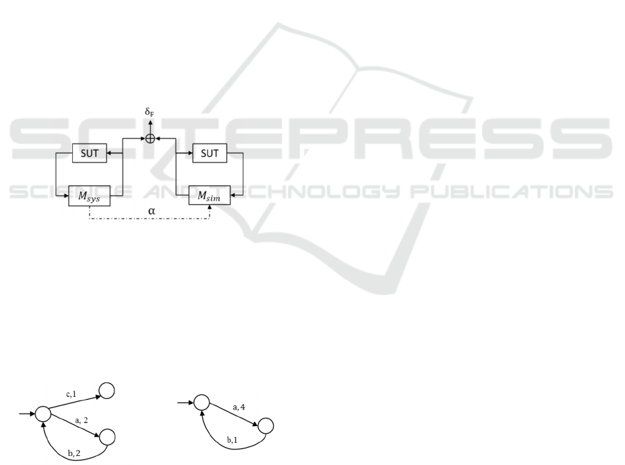
illustrated in figure 1. This quantification is absolute
if it is done independent of test cases i.e. some subset
of all possible stimulants and relative if it is done with
respect to the test cases. In this paper absolute fidelity
is discussed and this would intuitively mean that for
all possible inputs, the simulation model behaves
(within certain bounds) same as that of the system
such that the SUT could not see differentiate among
them.
Figure 1: Simulation Fidelity.
Let us consider a system specification given by
the system designer and a candidate simulation model
as shown in figure below. The dynamics are modeled
as a finite labeled timed transition system where for
example, from initial state upon receiving a label ‘a’
the system moves to the next state in 2 time units and
so on.
(a) System Model (b) Simulation Model
Figure 2: System & Simulation Model.
Consider a scenario where the simulation user
requires a simulation model with at least 80% fidelity
i.e. it is required to capture the transitions with 80%
(timing) accuracy. For the sake of simplicity, consider
the labels of two models are same and they differ only
with the time. A model developer, who is tasked with
developing or reusing an existing model needs to
quantify the model vis à vis this system specification
before integrating with other model fragments and
deploying on a platform. The objective in this case is
to measure the timing difference for each transition
and doing for all possible combinations yields a
formal fidelity measure. Recalling fidelity is the
ability of a model to match every move of the system
to the desired degree of accuracy, a two player game
can be played between them. In this game the first
player also called an attacker plays the role of system
whereas the second player also called defender plays
the role of simulation model. A model is said to be
with sufficient fidelity if the defender wins the game
with an acceptable degree of accuracy. In other
words, every move of attacker is matched by the
defender at the same time. In the given example, first
the attacker makes a move with either label ‘c’ at 1s
or ‘a’ at 2s. For the ‘c’ move, there exists no counter
move by the defender and the game is lost. On the
other hand, for the label ‘a’ move by attacker,
defender responds with same label in 4s and the time
cheat is 2s. For the next move of attacker with ‘b’
label at 2s, defender’s response is 1s and the time
cheat is -1s. The net timing error is then 1s at the end
of two transitions and this error increases linearly for
every loop made by the attacker on system model.
The resulting timing errors between the
corresponding transitions are evaluated against the
user requirement at the end to determine the model
adequacy. In the next section, these informal game
notions are formally presented using the quantitative
simulation relations based on two player game theory.
2.1 Quantitative Simulation Relations
In (reactive) systems modelling, the behaviour
exhibited by the system could be interpreted as a
sequence of letters representing observable events
collected as a language. A system’s behaviour can
then be checked against its requirement, both
specified as ω automaton by comparing their
languages. This linear view of checking language,
also called language inclusion is PSPACE hard for
finite state machines (Henzinger, 2013). On the other
hand, in a branching time view where the behaviours
are captured through tree automata, the algorithmic
complexity is only polynomial time. Simulation
relations (Alur et al., 1998), which relates two
systems based on this branching view, gives a
sufficient (but not necessary) condition to check this
Quantifying Fidelity for Timed Transition Systems
319

language inclusion between two automata. In this
paper, quantitative extensions of classical boolean
simulation relations proposed in (Cerny et al., 2010)
are used in the context of simulation fidelity i.e. to
quantify the degree of similarity between the
transition timings of system and simulation model.
Originally intended for software verification
where a program implementation is compared against
a specification, it is natural to extend this paradigm to
the domain of simulation where a model could be
interpreted as an implementation of a system
specification. This would mean evaluation of all
possible behaviours of a system specification against
a model i.e. absolute fidelity. In practice, only a
subset of the system’s state space is explored based
on a V&V plan and only such trajectories need be
reproduced by the model with adequate accuracy i.e.
relative fidelity. This could be factored in our
approach by relatively measuring this distance with
respect to the trajectories which are part of the V&V
plan and this is briefly discussed at the end of section
4. It may be noted that a truly absolute measure of
fidelity is with respect to the reality which is neither
feasible nor useful and hence in our study system
specification is assumed correct and approximated to
be the real system. In the following section some
preliminaries are explained.
2.1.1 Timed Simulation Relations
Let us consider the time domain with non-negative
set of reals
and over this time domain define the
timed automata (Alur and Dill, 1994) is defined by
,,,
,,, where is a finite non-
empty set of alphabets or labels, X is the finite non-
empty set of states, is a finite set of clocks,
⊆
is the initial non-empty state set, :⨯⨯→2
is the transition function and ⊆ X is the set of
accepting states. An accepting run of over a finite
word ꙍ=
…∈ is the sequence of states
…∈ such that
∈
. Then the language of
, is the set of words accepted by .
Let us consider two transition systems,
,
,
,
,
and
,
,
,
,
, with
∈
,
∈
, then
simulates
is denoted by
≼
and it holds if there exists a binary relation
⊆
such that if
,
∈ then
∀
,
,
∃
,
,
such that
,
∈
(1)
and it becomes bisimulation,
when
∀
,
,
∃
,
,
such that
,
∈
(2)
These simulation relations are usually boolean i.e. a
simulation model either simulates the system or not.
Quantitative extensions of these boolean notions are
based on finite-state turn based two player game
graphs. Two player game theoretic notions have been
used in verification as well as synthesis perspectives
in the formal modeling and analysis of systems
(Henzinger, 2013).
2.1.2 Timed Simulation Games
The two player turn based game is briefly introduced
in this section followed by the game between the
system and simulation model in the context of
quantifying its degree of similarity i.e. fidelity. A
game graph is a tuple, = <,
,
,,
> where
a finite set of states is partitioned as
and
for
the first and second player respectively such that
⋃
X,
⋂
∅, ⊆⨯ is the set of
edges,
is the initial state of the play (Alur et al.,
1998). The dynamics of the transition system
described by its states and transitions are interpreted
as nodes i.e. states and edges of this game.
The untimed game starts from state
∈ with a
player 1 making the move to
∈
to which the
player 2 counters by making a move
∈
. The
first play is over now and the game is started again.
At the end of first play, if the player 2 cannot match
player 1’s move it is allowed to cheat (Cerny et al.,
2010) and in doing so incurs a penalty and there are
different ways of measuring this cheat such as
weighted mean etc. This cheat measure gives a metric
on the degree of similarity between two models and
used in generating quantitative reachability for
untimed labelled transition systems in (Ponnusamy et
al., 2016). In this case of untimed or time-abstract
fidelity games, player 1 plays on the system model
and player 2 plays on the simulation model. Every
move on the system model by the first player is
followed by the second player on simulation model
and this continues until one wins. In particular, a
simulation relation exists if player 2 always has the
winning strategy. The strategy of the player to choose
each move may or may not depend on the history of
previous moves and in this paper we employ the
memory-less strategy. The set of visited states in the
game is called a play which is denoted by
…
and this is akin to the path of a transition system or
trace if there is a propositional evaluation at each such
state.
However, in timed game, the turn based nature of
the game does not strictly hold true due to the
temporal nature. The evolution of player 1 is
independent of the player 2 since the objective of
player 2 is to match player 1 timings. In other words,
player 2 is not allowed to win by infinitely blocking
SIMULTECH 2016 - 6th International Conference on Simulation and Modeling Methodologies, Technologies and Applications
320
the player 1’s turn (Chatain et al., 2009) whereas it
wait until player 1 finishes its turn.
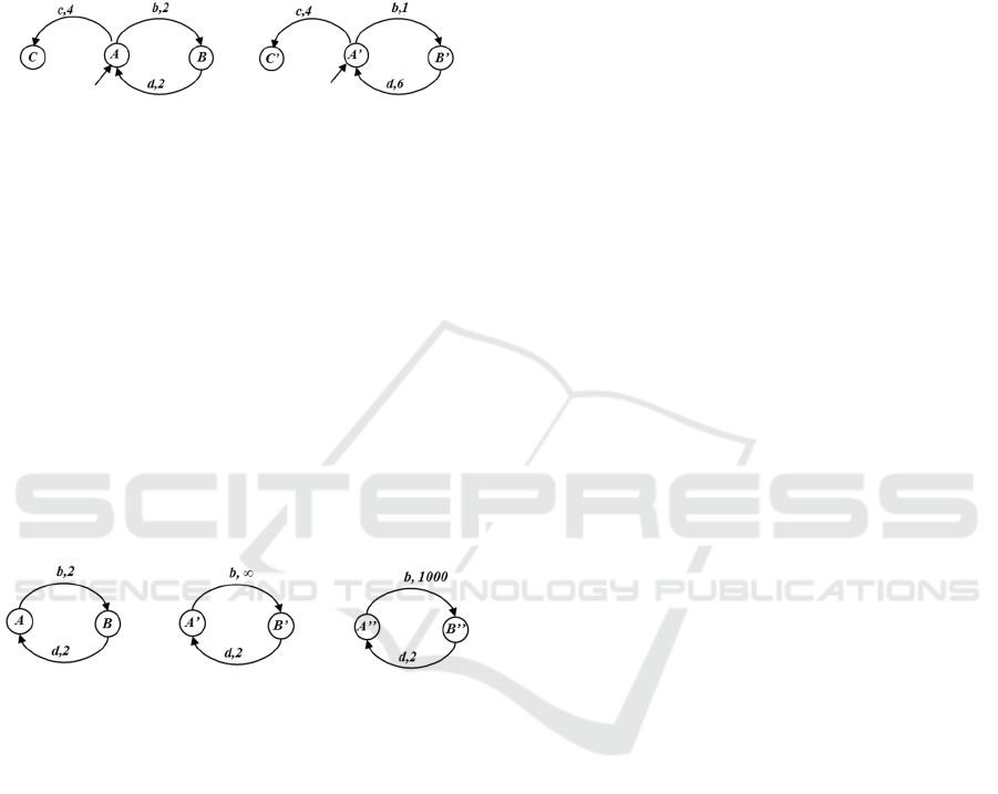
Proposition 1: Player 1 can block player 2’s time
Let us assume a system and simulation model in the
figure 3 and recall player 1 plays on
whereas
player 2 plays on
.
(a)
(b)
Figure 3: Blocking Game.
In this case, without blocking, player 2 label ‘b’ is
fired earlier and if player 1 moves ‘c’ instead, there is
a cheat whereas in reality the player 2 does not cheat
for ‘c’ transition. The blockage of time helps to avoid
this problem. Intuitively, a simulation model has to
mimic system model so it has to see what the system
does first or else it may end up in cheating even if a
way not to cheat exists.
Proposition 2: Player 2 cannot block player 1’s time
This assumption, also found in literature (Chatain et
al., 2009), could be explained with the following
example of game between a system and simulation
model in the figure below,
(a)
(b)
(c)
Figure 4: Non-blocking Game.
In this case, the third model is a better
approximation of the first model than the second.
However, if the game is played for <1002 time units
both the simulation models are deemed unfit and the
system model cannot move further from state B. This
can be mitigated by segregating the evolution of
system model from that of simulation model. In such
case, the time difference is 998 time units for the third
model and ∞ for the second model.
Then, formally, the game between system, M
and simulation model, M
is denoted by
M
,M
with the state space, X
⨯X
.
Let
,
be label and
,
be associated transition time
and of player 1 and 2 respectively at play i,
∈
and
∈
, player actions of selecting a
transition from one model and handing over the turn
to other player i.e. enabling transition of the other
model are denoted by
:
⟶
and
:
⟶
. For a given play of positive
integers, i∈
, player 1 move is defined as follows,
x
,τ
,x
→x
,τ
,x
(3)
with the transition time of simulation model
t
t
t
|t
t
if t
t
(4)
where t
is the blocked time
for player 2.
Then the
player 2 move is defined as
x
,τ
,x
→x
,τ
,x
if
σ
σ
t
t
(5)
The play is terminated if
σ
σ
regardless of their
transition times and the player 1 is deemed won. In all
other cases, the next play, i+1, is started with player
1 move if
t
t
.
At the end of each completed play,
the time difference between the corresponding
transitions i.e. labels,
∆t
is calculated using,
∆t
t
t
t
(6)
It may also be seen that such error function being a
directed metric (Chatterjee and Prabhu, 2015)
satisfies the reflexivity and triangular inequality i.e.
for all,
∆t
(
,
)=0 and
∆t
(
,
) ≤
∆t
(
,
) +
∆t
(
,
) respectively. This helps in incremental
model development and assembly with bounded
timing error on the resulting composition.
The timing error quantification through this game
based approach can be extended to system and/or
simulation models whose transition timings are not
defined precisely but in an interval as well. Let us
define such interval for the system and simulation
model as [
,
,
] where lb and ub refers to lower
and upper bounds on transition timings. In this case,
intuitively the interval difference is the timing
difference and Eq.4 becomes,
t
t
t
|t
t
if t
t
(7)
where t
is the blocked time
for player 2. In other
words, the transition of player 2 is enabled once
player 1’s lower bound transition time is enabled.
Then the interval timing error,
∆
∆
is
calculated
as,
∆
t
t
t
∆
t
t
t
(8)
Quantifying Fidelity for Timed Transition Systems
321

However, such interval error quantification needs
to be further studied and is not yet implemented in our
tool and only transitions fired at punctual time i.e.
,
,
is considered in this study.
In discussing fidelity quantification through such
game based approach, one of the key difficulties is
exploring the player’s strategies. Instead of a
simulation approach, which is semi-formal and often
error prone, a formal method of exploring all such
player strategies is needed. In this context, a
reachability graph generation which explores all the
player’s strategies to quantitatively determine the
corresponding transition timings is presented in the
next section.
2.2 Quantitative Reachability
Reachability, in general, is the problem of
determining the existence of a trajectory that visits a
state. An exhaustive exploration of all such
trajectories results in a reachability set, which is
usually verified against some boolean specification
such as safety and this process is called model
checking. Since timed games generate a quantitative
measure for each trace of the simulation model vis à
vis the system model, generating a reachability set of
these timed games result in a formal and quantifiable
reachability set. In other words, this is an exhaustive
exploration of all the player strategies. However, in
contrast to untimed games, continuous evolution of
time for the attacker and blocking for the defender
need to be taken into account in the play and error
quantification as well.
A key benefit of such formal approach is the
global distribution of fidelity in terms of event
timings with respect to the system model. Such
quantitative graphs can be analyzed to determine the
optimal strategies, least or maximum error paths etc.
In practice, simulation models are usually not
developed from scratch but built by reusing the
existing model fragments from a library. In such
cases, the global distribution of fidelity could be
analyzed to determine the adequacy of a particular
model for the given test case.
The (pseudo) reachability graph is illustrated in
figure 5 for games described in section 2 and figure
2. The transitions of attacker and defender are given
in solid and dotted arrows respectively. The first play
is over at 6s and the second play is over at 7s and it
can be seen that the blocking time is 2s. In addition,
due to the absence of a matching transition for
attacker move on ‘c’ label, the game is locally lost on
this path.
Figure 5: Quantitative Timed Reachability Graph.
Then the timing error is calculated as
∆
62
22
and
∆
72
50
and so on. It can be
easily seen that the pair-wise timing error can be
deducted from this aggregate time, for example, the
timing difference for second turn is -2. Such evolution
can be analyzed and visualized for better
understanding of the model fidelity.
3 IMPLEMENTATION
The game semantics and reachability generation
discussed in section 2 is implemented in the Petri-Net
formalism. Timed petri-net is an extension of
classical petri-net formalism (Berthomieu and Diaz,
1991) with firing time for the events. Such formalism
is widely used to represent the timed execution of
discrete event systems interleaved with (possibly
zero) delays. Formally, a petri-net is a tuple
,,,,
,
(9)
where
- P is a finite set of symbols called places
- is a finite set of symbols called (timed)
transitions with P ∩ = ∅
- ⊆ (×P) ∪(P×)
is the set of arcs defining the
flow relation
-
: → N
is the function defining the respective
weights of the arcs, N=1 in our case
-
:
→
is static interval function with
,
the
non-empty set of positive real intervals including 0.
-
: P → N
is the initial marking
Informally a transition, is enabled if there is a
token at the corresponding place,
∈
and moves to
the next state defined by the flow relation. This token
and place formalism of Petri-net is amenable to model
the two player turn-based game which is alternating
in terms of player turns. In the current study no
concurrency is assumed and the resulting games have
only total states. A state s of a Petri net is a couple
,
where m is the marking and I is the interval
SIMULTECH 2016 - 6th International Conference on Simulation and Modeling Methodologies, Technologies and Applications
322
function,
:
→
which associates to each enabled
transition at marking m a temporal interval. In
addition, only intervals under the form [θ,θ], i.e.
deterministic event timings are considered although
firing at timings drawn randomly from uniform
distribution is also possible.
3.1 Tool Implementation
The game semantics described in previous sections has
been implemented in TINA, a (un)timed petri-net
editor and analysis tool used to generate marked
reachability graph,
for timed systems through state
classes (Berthomieu and Diaz, 1991). This game
semantics is then integrated into ProDEVS, a
simulation platform for systems modeled in Discrete
EVent Specification (DEVS) formalism, (un)timed
classical automata and untimed interface automata
(Vu,2015). The system and simulation models are
constructed as timed automata in ProDEVS. In
addition, it may be noted that DEVS is akin to timed
interface automata which is essentially finite state
automaton with embedded time and differentiation
between input and output labels. DEVS, whose
definitions can be found in (Zeigler et al., 2000) is a
hierarchical and modular formalism used to model
discrete, continuous and hybrid timed transition
systems. Since we intend to extend the current
quantitative approach to timed interface automata from
the existing timed automata, models are constructed in
ProDEVS itself. These models are then converted to
equivalent timed petri-net models in TINA. The game
is automatically constructed between them in TINA-
ND editor and the reachability graph is generated. It
may be noted that since petri-net simulator per se does
not handle data, these are encoded as guards and
actions on the transitions through associated c files to
generate dll files to be run by TINA. This graph in text
form is then parsed in ProDEVS to perform some
analytics for better understanding and visualization.
The ProDEVS parser constructs a reachability tree
which can then be visualized and plots the evolution of
cheats along the play, distribution of cheats etc. The
replay feature allows to choose a particular cheat from
the cheat distribution plot to see the associated path to
better understand when and where the simulation
model behaviour differs with respect to the system.
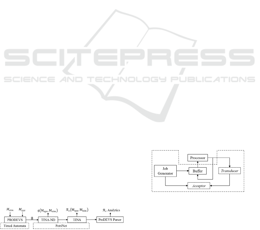
The overall methodology is illustrated in the
figure below.
Figure 6: Implementation.
It can be seen that the modeling and parsing are
done in ProDEVS with rest being in TINA.
Alternatively, modeling and reachability generation
could be done directly in TINA as well and ProDEVS
could then be used to simply parse the data. It may be
seen that, given a system design model and a
simulation model, the game is constructed
automatically and the resulting output is exhaustive
timing error quantification over all possible transitions.
The simulation user or the developer may then decide
to improve the simulation model or relax the V&V
requirements. This approach, apart from quantifying
the global fidelity independent of V&V objectives, is
also useful in iteratively refining the design with
respect to V&V scenarios especially in the early
system development when the design is not frozen.
4 APPLICATION CASE
The application case considered is a simple FIFO
buffer which is connected to a job generator and a
processor. The buffer system model is shown in
figure 7 where it receives the job, e0 from generator
and sends it to the processor, s0 with the associated
number of jobs stored in a queue variable, q. In
addition, the buffer sends the job based on the
processor status, e1. Let the processor be the SUT
under some user defined scenarios,
..
. This
scenario of experimentation is illustrated using the
experimental frame formalism (Zeigler et al., 2000)
where the SUT and the environment systems such as
buffer and generator need to perform this validation
activity could be seen. In addition, such experimental
frame may contain transducer and acceptor which are
used for interpretation and validation of experimental
frame component’s outputs. For example, a
transducer might convert processor status as number
of processed jobs which will then be compared
against the generated jobs.
Figure 7: Buffer Model for Processor Validation.
In validating the buffer through simulation, a
model of its environment, in this case the buffer, need
to be modelled with a quantifiable degree of fidelity.
Let us consider the buffer system specification,
Quantifying Fidelity for Timed Transition Systems
323
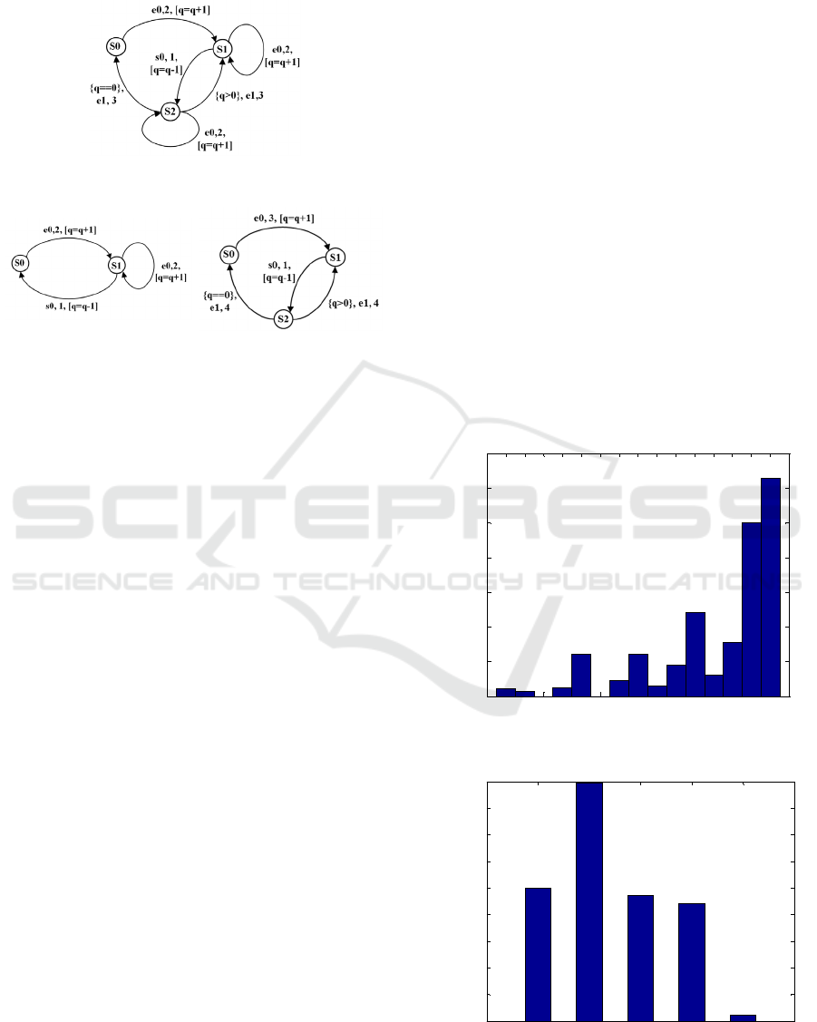
and two simulation models of the system,
,
as
shown in figure 8 and 9 respectively.
Figure 8: Buffer System Model.
(a)
(b)
Figure 9: Buffer Simulation Model.
The transition labels are typically given in the form of
tuple <{}, ,
t, []>
where {},[] refers to guards and
actions respectively. In this case, the guards and
actions are on the queue variable, q.
This game can be either played state bounded or
equivalently play bounded. In the former, the
maximum number of state classes generated during
reachability construction is fixed whereas in the latter
the play is terminated only if all the winning
trajectories (if it exists) where
σ
σ
of player 2 are
played. In addition, a play can be terminated
prematurely if the number of lost trajectories exceeds
a certain user defined bound. Different such
techniques could be employed to manage the game
and interpret the results to determine the fidelity
according to the user requirement. In the following
section some fidelity metrics are discussed for the
buffer model.
4.1 Analysis Results
The timed fidelity game is played between
and
and a quantitative reachability graph is generated
for a maximum 10
3
state classes. Since the size of
is
limited, the first question is how many traces are
generated and how long they are i.e. length. In total
4661 traces were generated with 3640 traces has
maximum trace length of 26 transitions. It may be
reminded that in this case, the system model makes
infinite number of turns regardless of the simulation
model and incompleteness of each trace is
predominantly due to the truncation of reachability
states generated. The distribution of all such transitions
can be visualised in figure 10. It can be seen that most
traces have one or two transitions empty due to
reachability graph truncation and this information can
be used to limit or extend the limit of exploration.
For each trace, the number of plays may be
different i.e. a play might be lost but still the trace
contains only player 1’s transitions. It can be seen
from figure 11 that simulation model can match the
transition labels for a maximum of 5 plays for 45
traces. For each of these traces, associated timing
error can be extracted similar to figure 5.
For example, the trace with transition sequence
0
→0
→1
→0
→0
→1
of system model can be
matched by the corresponding sequence
0
→0
→1
→
0
→0
→1
of the simulation model and the net timing
error is 3 time units at the end of fifth play. However,
for some other traces it can match only partially, for
example one can intuitively see that a job can arrive at
any state for the system model whereas the simulation
model can take job only at state S0. In such traces, (e.g.
0
→0
→0
→…
by the system
)
the game is partially lost
and such information too can be obtained.
Figure 10: Trace length vs Number of traces.
Figure 11: Total number of plays distribution.
11 12 13 14 15 16 17 18 19 20 21 22 23 24 25
0
50
100
150
200
250
300
350
Trace Length
Number of traces
0 1 2 3 4 5 6
0
200
400
600
800
1000
1200
1400
1600
1800
Number of Plays
Number of Traces
SIMULTECH 2016 - 6th International Conference on Simulation and Modeling Methodologies, Technologies and Applications
324
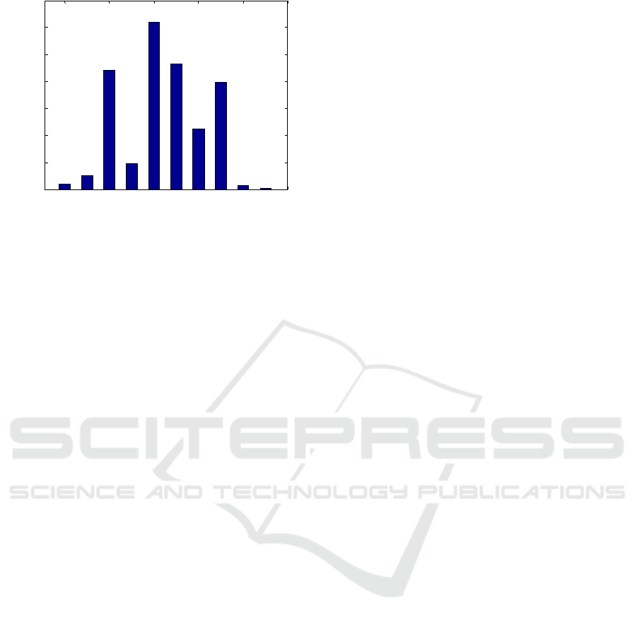
Figure 12: Transition difference distribution.
Another key information of interest is the lead
information i.e. how far the system is in advance
before the simulation model and this represents the
overall lag of the simulation model with respect to
system. A near perfect simulation model has less lag
and increase in lag is either due to the play being lost
in that trace especially for systems with loops such as
buffer or simulation model timings are higher. The
figure 12 shows this difference and it can be seen that
almost all lag is due to the play being lost in
corresponding traces. At maximum only one
transition i.e. e0 is matched for 995 traces.
A key aspect which is not discussed is the role of
V&V objectives in this fidelity quantification. In the
current study, all the differences in transition timings
are equally weighed. However, in reality a model is
developed with some V&V objectives behind and in
such cases some transitions are of more interest than
the others. Let us consider a requirement,
1
on SUT
stating that all the sent jobs must be processed by the
processor i.e. no job is lost. In other words, an ideal
buffer must store and send the jobs to processor as a
function of processor status. In case of first simulation
model this is not true as the processor status is not
modeled. This is characterised by the losing game in
the third play of the game whenever the system makes
a move with e1 label. However, in case of second
simulation model the game is not lost but the event
timings are different. On the other hand, consider
requirement,
2
on SUT stating processor expects at
least one job at delivered by the buffer at 3s and in
this case first simulation model matches exactly the
transition timings
0
→0
→0 compared to the
.
Thus, depending on the requirement, some transition
timings are weighed more with weighting
, than the
others with weighting
, in which case the
complexity of the method is increased to
|
||
|||
||.
5 OUTLOOK & CONCLUSIONS
A formal quantitative approach to simulation fidelity
based on simulation relations and two player game is
presented. Our contribution is threefold, first,
extending timed games into a fidelity problem,
mapping this game in petri-net formalism, generation
of quantitative reachability and analysis with some
fidelity metrics. However, this explicit enumeration
of traces along with their (timing) distances may
suffer from the curse of dimensionality and of limited
use in large scale systems. This may be mitigated by
using efficient data structures such as using Binary
Decision Diagrams (BDD) and studies need to be
made in abstraction, and abstraction refinement
techniques, especially for continuous systems.
Another practical challenge is the availability of the
system specification, especially in formal language
such as timed automata. Even in case of such
availability, there could be interoperability issues
between the modelling formalisms used by the model
developer and the system designer. In addition, the
current study concerns only timed automata which
does not differentiate between the labels i.e. inputs
and outputs and does not capture the environment
assumptions. This study is currently being extended
to interface automata and an untimed distance notion
for interface automata (Cerny et al., 2014) has been
implemented in ProDEVS. An extension to timed
interface automata is being studied which will enable
fidelity quantification of the DEVS systems.
The quantitative perspective discussed in the
paper will enable different stakeholders in the system
V&V process to develop and reuse models with a
known and assured level of fidelity. For example, the
model developer could gain key insights into the
model behaviour and chooses the best abstraction of
the system vis à vis the scenario. On the other hand,
the system test team would have a measure of fitness
on the models being used for the V&V which would
mitigate unfeasible or unclear model fidelity
requirements. In addition, this would benefit the
system designer in making improvements or
modifications to the system model. These benefits
would allow not only to select a consistent model with
sufficient level of fidelity according to the test case
with different criteria such as performance,
robustness etc. but also to help in quantifying the
fidelity of the overall V&V process. Such a
quantitative framework to fidelity will enable
significant benefits in avoiding redundant modelling
and validation effort thereby saving cost and time in
product development especially in replacing real tests
with simulation i.e. virtual testing.
0 2 4 6 8 10
0
200
400
600
800
1000
1200
1400
Transition Difference
Number of Traces
Quantifying Fidelity for Timed Transition Systems
325

ACKNOWLEDGEMENTS
The authors would like to thank Bernard Berthomieu
of CNRS, LAAS for his contribution in using
FIACRE and TINA for this study.
REFERENCES
Albert, V., Ponnusamy, S.S., 2016, Encoding CDEVS and
PDEVS into Timed Petri Net: theory and application,
Journées DEVS Francophones, Accepted.
Alfaro, L., Faella, M., Stoelinga, M., 2009, Linear and
Branching System Metrics, IEEE Trans. Software Eng,
Vol 35(2), 258–273.
Alur, R., Henzinger, T., Kupferman, O., Vardi, M., 1998
Alternating refinement relations. Lecture Notes in
Computer Science, Vol 1466, 163-178.
Alur, R., and Dill, D., 1994, A theory of timed automata,
Theoretical Computer Science, Vol 126,183–235.
Brade D, VV&A Global Taxonomy (TAXO), 2004,
Common Validation, Verification and Accreditation
Framework for Simulation, REVVA.
Berthomieu, B., Diaz, M., 1991, Modeling and verification
of time dependent systems using time Petri nets, IEEE
Trans on Software Engineering, Vol. 17, no. 3, 259-
273.
Cerny,P., Henzinger, T. & Radhakrishna, A., 2014,
Interface simulation distances. Theoretical Computer
Science, Vol 560, 348-363.
Cerny,P., Henzinger, T. & Radhakrishna, A., 2010,
Simulation Distances, Lecture Notes in Computer
Science, Vol 6269, 253–268.
Chatain, T., David, A., Larsen, K.G., 2009, Playing games
with timed games, Proceedings of the 3rd IFAC
Conference on Analysis and Design of Hybrid Systems,
Zaragoza, Spain.
Chatterjee, K., Prabhu,V.S., 2015, Quantitative Temporal
Simulation and Refinement Distances for Timed
Systems, IEEE Transactions on Automatic Control, Vol
60, Issue 9, 2291-2306.
Girard, A., Pappas, G.J., 2007, Approximation Metrics for
Discrete and Continuous Systems. IEEE Transactions
on Automatic Control, Vol 52, Issue 5, 782-798.
Henzinger, T. A., 2013, Quantitative reactive modeling and
verification, Journal of Computer Science Research
and Development, Vol 28 Issue 4, 331-344.
Ponnusamy, S.S., Thebault P., Albert V., 2016, Simulation
Fidleity-A Game Theoretic Approach, Spring
Simulation Multi-Conference, US, Accepted.
Ponnusamy S.S., Albert V., Thebault P., 2014. A simulation
fidelity assessment framework. International
Conference on Simulation and Modeling
Methodologies, Technologies and Applications, pages
463-471, Vienne, Austria.
Roza M., 1999. Fidelity Requirements Specification: A
Process Oriented View. Fall Simulation
Interoperability Workshop.
Vu, L.H., Foures, D., Albert, V., 2015, ProDEVS: an event-
driven modeling and simulation tool for hybrid systems
using state diagrams, Proceedings of the 8th
International Conference on Simulation Tools and
Techniques, 29-37, Greece.
Zeigler, B.P., Praehofer, H., Tag, G.K., 2000,
Theory of
modeling and simulation, San Diego, California, USA.
Academic Press.
SIMULTECH 2016 - 6th International Conference on Simulation and Modeling Methodologies, Technologies and Applications
326
