Generalized Disturbance Estimation via ESLKF for the Motion Control
of Rotorcraft Having a Rod-suspended Load
J. Escareno
1,2
, A. Belbachir
1
, T. Raharijaona
3
and S. Bouchafa
2
1
Institut Polytechnique des Sciences Avanc
´
ees, 194200 Ivry sur Seine, France
2
Universit
´
e d’Evry, Laboratoire IBISC, 91020 Evry, France
3
Aix-Marseille Universit
´
e, CNRS, ISM UMR 7287, 13288 Marseille Cedex 09, France
Keywords:
Multi-body Rotorcrafts, Linear Kalman Filter, Extended-state Estimation, Robust Navigation, Hierachical
Control, Time-scale Separation.
Abstract:
The aim of the paper is to propose a navigation strategy applied to a class of rotorcraft having a free rod-
suspended load. The presented approach relies on the Linear Kalman Filter to estimate the not only the state
vector but also a generalized disturbance term containing parametric, couplings and external uncertainties.
A simple hierarchical control is used to drive the motion of the rotorcraft, which is thus updated with the
estimation of the disturbance evolving during the a navigation task. Despite the time-scale separation due to
the underactuated nature of the flying robot, the estimation approach has shown its effectiveness considering
the same sampling time. A detailed simulation model is used to evaluate the performance of the proposal
under different disturbed scenarios.
1 INTRODUCTION
In the last years the Unmanned Aerial Vehicles
(UAVs), specially miniature aerial vehicles (MAVs)
were used for a wide variety of tasks either indus-
trial or scientific. The operational capabilities of these
aerial vehicles are evolving and thus novel applica-
tions are arising. The technological and scientific
challenges associated to this emergent generation of
aerial robots are enormous. The aerial interactivity
with the environment is a trendy MAV-based applica-
tions category, whose most notorious examples are in-
contact structure inspection, aerial manipulation and
transportation.
The dynamic structure of a rotorcraft endowed
with a rod-suspended load, either rigidly attached to
airframe (robotic arm) or freely rotating pendulum
(rod cable-suspended load) , can be considered as a
general case for aerial manipulation and transporta-
tion. Several works have been proposed in such top-
ics. In (Bernard et al., 2010), the problem of slung
load transportation using autonomous small size he-
licopters is addressed. The Newton-Euler modeling
and control of a variable number of helicopters trans-
porting a load is presented. Indeed, the proposed
controller prevents and compensates oscillations of
load during the flight, which is demonstrated by real
flight load transportation by three helicopters. On
the other hand in the case of rotorcrafts mini aerial
vehicles (MAVs), they features a reduced payload-
carrying capacity which represents an critical issue
while transporting cargo or aerial grasping. How-
ever, multiple vehicles are able to overcome this is-
sue, as demostrated (Mellinger et al., 2010), where
a quad-rotors fleet transport a cargo through cables.
The generation of trajectories where the quadrotor
provides swing-free load motion has attracted the in-
terest of diverse authors. In (Palunko et al., 2012)
is presented the strategy to generate trajectories that
provides a swing-free load’s motion. In (Faust et al.,
2013) the same problem is addressed using a rein-
forcement learning algorithm to reduce loads oscilla-
tions. Sharing the same objective, in (Cruz and Fierro,
2014) a geometric control is proposed. An alternative
UAV configuration equipped with a hook intended to
deliver/retriving cargo using a vision-based strategy is
presented in (Kuntz and Oh, 2008). Likewise, various
contributions can be found on the literature regard-
ing the aerial grasping and/or manipulation. (Pounds
et al., 2011) presents the planar model, attitude con-
trol analysis and outdoors experimental validation of
a middle-size helicopter equipped with a compliant
gripper capable of robust grasping and transporting
objects of different shapes and dimensions. In (Gha-
526
Escareno, J., Belbachir, A., Raharijaona, T. and Bouchafa, S.
Generalized Disturbance Estimation via ESLKF for the Motion Control of Rotorcraft Having a Rod-suspended Load.
DOI: 10.5220/0006009105260533
In Proceedings of the 13th International Conference on Informatics in Control, Automation and Robotics (ICINCO 2016) - Volume 2, pages 526-533
ISBN: 978-989-758-198-4
Copyright
c
 2016 by SCITEPRESS – Science and Technology Publications, Lda. All rights reserved

diok and Ren, 2012), a classical quadrotor featuring
a home-customized 1DOF gripper performs an aerial
grasping based IR camera. In (Ghadiok and Ren,
), the experiments are extended to outdoor, using a
GPS system and a Kalman filter to improve the pre-
cision in the position system. Both contributions use
a customized 1-DOF gripper. (Yeol and Lin, 2014)
presents a quadrotor equipped with a four-fingered
gripper which enables to perform aerial grasping and
perching. The gripper is directly attached to the vehi-
cle, this fact restricts the grasping workspace, i.e. the
vehicle’s center of mass (CoM) must be aligned to
the object to be grasped (target). From the mechani-
cal point of view, the gripper is signficately complex
featuring 16 DOF, 4 joints per finger. In (Thomas
et al., 2014), the authors present a classical quadro-
tor equipped with a monocular camera. The pro-
posed control strategy enables performing aggressive
grasping maneuvers via an Image Based Visual Ser-
voing (IBVS). It is claimed that unlike most IBVS
approaches, the dynamics is obtained directly in the
image to deal with a second order system. In (Pizetta
et al., 2015) it is presented the modeling and bounded
control of a quadrotor having a suspended load. In
this case the dynamic couplings are considered only
in the translational subsystem of the aerial robot, and
the pitch dynamics lacks of dynamic couplings. This
simplifies the control task since the underactuated na-
ture of the overall rotorcraft’s motion relies on the
pitch control effectiveness.
While most of the contributions, related with sus-
pended load, focuses on the trajectory generation to
attain a swing-free motion, in the current paper we
prioritize the navigation stability of the rotorcraft re-
gardless the dynamic disturbances resulting from the
coupling with the motion of a freely rotating pen-
dulum (aerial pendulum) which is also vulnerable to
external disturbances, which. The paper provides
a detailed description of the dynamic model, which
is obtained through the Euler-Lagrange formalism.
The rotorcraft model is represented as disturbed sys-
tem, affected by the couplings with aerial pendulum.
We have based our estimation approach on the Lin-
ear Kalman Filter (LKF), whose framework allows
to define extended states to take into account the un-
known inputs. In this regard, the LKF is applied
in both dynamic layers, the rotational and transla-
tional, which feature a nonlinear underactuated dy-
namic structure. Despite the time-scale separation be-
tween such dynamics, the LKF is implemented con-
sidering the same sampling-time.
The paper is organized as follows. Section 1 de-
scribe the context and previous works of the herein
presented rotorcraft class the grasping problem is dis-

mrg
ey
T
mp
ez

ex
e2
e1
e3
mpg
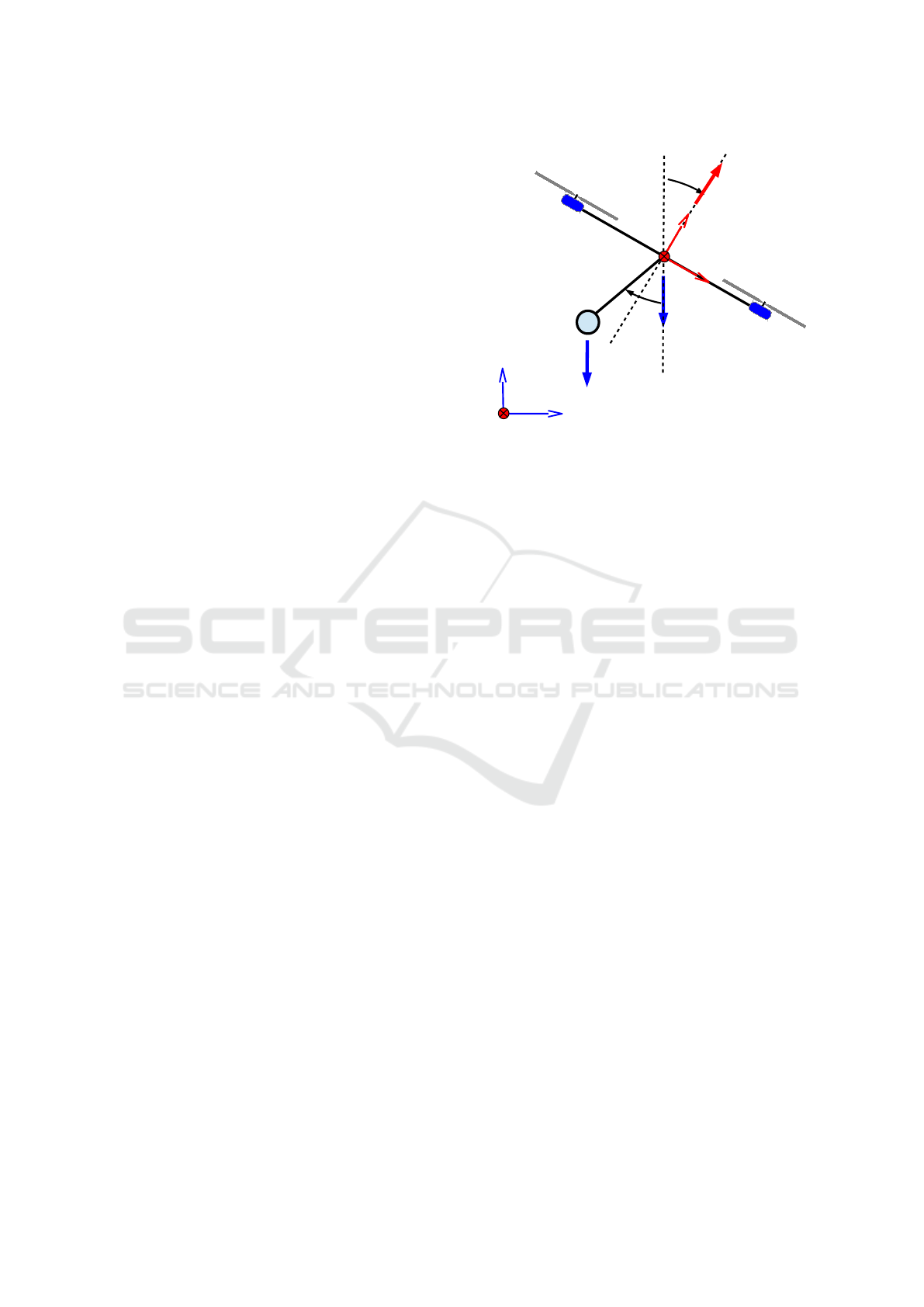
Figure 1: Drone Pendulum.
cussed. Section 2 details the mathematical model ob-
tained via the Euler-Lagrange. Section 3 and 4, de-
scribes the navigations strategy. Finally, section 5
provides the conclusions and future works.
2 DYNAMIC MODEL
Consider a rotorcraft, of mass m
r
∈ R, having a load
mass m
p
∈ R which is linked to the main airframe
through a massless rigid rod of length l
p
∈ R (aerial
pendulum). For the actual study and for the sake
of simplicity, the rotorcraft is restricted to evolve
within the longitudinal plane (see Fig.2). For such
class of vehicle, the general expressions that gov-
erns the dynamic behavior are obtained through the
Euler-Lagrange approach, such energy-based formal-
ism provides cross-linked couplings between the ro-
torcraft and the payload. Let θ ∈ R represent the pitch
angle, γ ∈ R the rod’s angle with respect to (w.r.t.)
−e
3
, while T
1
and T
2
denote the thrust force provided
by frontal and rear propellers, respectively. The in-
ertial frame is denoted by {I : (e
x
,e
yx
,e
z
)} and the
body-fixed frame is {B : (e
1
,e
2
,e
3
)} and the rota-
tion matrix relating the body frame with inertial is
R
θ
∈ SO(3) which corresponds and is given as The
equations of motion modeling a rotorcraft having a
free pendular mass represent a versatile model that
can be adapted or simplified for several multi-body
rotorcraft configurations. For instance, the current
trend of flying robots featuring actuated robotic ma-
nipulators can be considered as a vehicle sub-class
of the rod-load configuration. In this regard, diverse
nonlinear adverse terms, coupling and external dis-
turbances, arise during in-hovering grasping, manip-
ulation and surface-contact operations, affecting the
nominal moments and forces equations. Furthermore,
Generalized Disturbance Estimation via ESLKF for the Motion Control of Rotorcraft Having a Rod-suspended Load
527

couplings arise from translational motion and, obvi-
ously, due to vehicle’s underactuated nature, the rota-
tional motion.
In order to obtain the equations of motion through
the Euler-Lagrange, it is required the knowledge of
the kinetic and potential energies for the rotorcraft and
the rod-load mechanisms.
2.1 Kinetic Energy
The kinetic energy function of the rotorcraft is given,
K
r
=
1
2
I
r
˙
θ
2
+
1
2
m
r
˙x
2
+
1
2
m
r
˙z
2
. (1)
where I
r
denotes the inertia tensor of the rotorcraft.
Due coordinates of the pendular mass are shifted from
the body frame B, the kinetic energy of aerial pendu-
lum is written
K
p
=
1
2
m
p
˙x
2
p
+
1
2
m
p
˙z
2
p
(2)
where m
p
represents the pendular mass, and
˙x
p
= ˙x − l
p
˙
γcos γ
˙z
p
= ˙z + l
p
˙
γsin γ
,
are obtained from the cartesian coordinates follow a
right-handed rotation about e
2
x
p
= x − l
p
sinγ
z
p
= z − l
p
cosγ
,
Thus, the expression for the aerial pendulum is writ-
ten as
K
p
=
1
2
m
p
( ˙x − l
p
˙
γcos γ)
2
+
1
2
m
p
(˙z + l
p
˙
γsin γ)
2
. (3)
It is straightforward to reduce latter equation into
K
p
=
1
2
m
p
˙x +
1
2
m
p
˙z + ζ
c
( ˙x, ˙z,
˙
γ) +
1
2
m
p
I
p
˙
γ
2
, (4)
where ζ
c
energy coupling and is given
ζ
c
= m
p
l
p
˙
γ(− ˙x cos γ + ˙zsin γ). (5)
The total kinetic of the aerial multi-body system is
K = K
r
+ K
p
(6)
2.2 Potential Energy
The potential energy of the of the rotorcraft is ob-
tained as
P
r
= m
r
gz (7)
while that of the aerial pendulum is written as
P
p
= m
p
g(z − l
p
cosγ) (8)
The total potential energy is
P = P
r
+ P
p
(9)
2.3 Equations of Motion
The Lagrangian L ∈ R is L = K − P. Hence, in order
to obtain the equations of motion, the general Euler-
Lagrange equation is solved for the different general-
ized coordinates q = (x,z,θ, γ)
T
∈ R
4
d
dt

∂L
∂ ˙q

−
∂L
∂q
= U, (10)
where the control inputs vector U = (u
x
,u
z
,u
θ
,u
γ
)
T
=
(U
t
,U
r
)
T
. For the underactuated translational motion
subsystem, the rotational matrix angles the thrust vec-
tor T as
U
t
= R
θ
Te
3
= (T sin θ, T cos θ)
T
= (u
x
,u
z
)
T
(11)
is the thrust vectoring through pitch angle. Concern-
ing, the rotational motion control input,
U
r
= (u
θ
,u
γ
)
T
, (12)
one can notice that unlike rotorcraft’s attitude the
aerial pendulum is not actuated (i.e. u
r
= 0).
The equations of motion results from solving
Eq.10 for the different generalized coordinates. For
the translational motion, we obtain
(m
r
+ m
p
) ¨x − m
p
l
p
¨
γcos γ + m
p
l
p
˙
γ
2
sinγ = u
x
(13)
(m
r
+m
p
)¨z+ml
p
¨
γsin γ+m
p
l
p
˙
γ
2
cosγ+(m
r
+m
p
)g = u
z
(14)
The corresponding equations describing the rotational
motion of the rotorcraft and the aerial pendulum are
given next.
I
r
¨
θ = u
θ
(15)
and
m
p
l
2
p
¨
γ − m
p
l
p
¨x cos γ + ¨zm
p
l
p
sinγ + m
p
gl
p
sinγ = u
γ
(16)
where u
γ
= 0 since the aerial pendulum is in free mo-
tion.
Remark 2.1. It is important to point out that the
torques of the pendulum dynamics are also exerted
about the axis e
2
as the pitch dynamics. Thus, pitch
behavior is also impacted by the pendulum’s torques
2.4 Disturbed System
The equations (Eq.13-Eq.16) obtained from the Euler-
Lagrange formulation (Eq.10), are rewritten in order
to represent coupled system as disturbed system. In
this representation, the coupling terms are considered
as disturbances since they are assumed unknown. In
this regard, the mass of the pendulum is unknown but
verifying
m
p
< m
r
(17)
ICINCO 2016 - 13th International Conference on Informatics in Control, Automation and Robotics
528

The equations describing the horizontal motion are
rewritten as follows:
¨x =
1
m
r
(u
x
+ ρ
x
), (18)
with
ρ
x
= −m
p
¨x + m
p
l
p
¨
γcos γ − ml
p
˙
γ
2
sinγ (19)
whereas, the vertical motion is rewritten as
m
r
¨z =
1
m
r
(u
z
+ ρ
z
) − g, (20)
with
ρ
z
= −m
p
¨z − m
p
l
p
¨
γsin γ − m
p
l
p
˙
γ
2
cosγ − m
p
g (21)
One can notice that ρ
x
and ρ
z
corresponds to the tan-
gential, centrifugal and gravity-due forces generated
by the pendular motion of the mass m
p
. Even if the
torques of the rotorcraft and aerial pendulum are ex-
erted about the e
2
axis, the rotational motion of the of
the aerial pendulum is not affected (assuming µ = 0)
by that of the rotorcraft. However, this is not the case
for the rotorcraft rotational motion, which is affected
by the torques due the motion of the pendular motion
shifting the center of gravity of the rotorcraft. The lat-
ter allows us to rewrite the rotorcraft dynamics Eq.15
as:
¨
θ =
1
I
r
(u
θ
+ ρ
θ
) (22)
with
ρ
θ
= −m
p
l
p
¨
γ+ m
p
l
p
¨x cos β− ¨zm
p
l
p
sinβ −m
p
gl
p
sinγ
(23)
3 DISTURBANCE ESTIMATION
STRATEGY
An extended state discrete linear Kalman filter (ES-
LKF) is designed regarding the estimation of the cou-
plings and disturbances arising during a planar dis-
placement at rotational (inner dynamics) and transla-
tional (external dynamics) The Linear Kalman Filter
(LKF) is derived from a continuous system

˙x(t) = Ax(t) + Bu(t) + M ω(t) → process
y(t) = Cx(t) + ν(t) → sensor(s)
(24)
that considers the following hypothesis:
H1. The pair AC verifies the controllability property
H2. The signals α and β stand for a white Gaussian
random process with zero-mean (E [α(t)] = 0)
and E [β(t)] = 0)) with constant power spectral
density (PSD) W (t) and V (t) defining respec-
tively:
• The process covariance matrix
Q = E

α(t)α(t + τ)
T

= W ∆(τ) (25)
• The sensor covariance matrix
R = E

β(t)β(t + τ)
T

= V ∆(τ) (26)
It is also assumed that both stochastic processes are
not correlated, i.e.
E

α(t)β(t)
T

= 0 (27)
3.1 Extended-state Estimation Strategy
Since we are interested in the stability of the rotor-
craftThe kalman filter is applied to the rotorcraft. Let
us regroup the set of scalar disturbed systems Equ. 18,
Equ. 20 andEqu. 22.
¨
χ
i
=
1
a
i
(U
i
+ ρ
i
) − G
i
with i ∈ {x,z,θ} (28)
with
• G
x
= 0, G
z
= g and G
θ
= 0
•
¨
χ
x
= ¨x,
¨
χ
z
= ¨z and
¨
χ
θ
=
¨
θ
• a
x
= m
r
, a
z
= m
r
and a
θ
= I
r
In Equ. 28 we have included the G
i
term to keep the
general i−structure regrouping the three disturbed dy-
namics. The model Equ. 28 may be rewritten into the
space-state representation
˙
X = AX + B(u
i
− a
i
G
i
) + Pρ
i
Y = CX
(29)
having as a state and output vector
X = Y = (χ
i
,
˙
χ
i
)
T
= (χ
1
i
,χ
2
i
)
T
(30)
the latter indicates that translational and rotational po-
sitions and velocities are available. The vector ρ
i
uni-
fies the couplings and external disturbances. The ma-
trices of the system (Equ. 29) are given by:
A =

0 1
0 0

,B =

0
a
i

,P =

0
a
i

,C =

1 0
0 1

,
(31)
It is assumed that no prior information about the dis-
turbance is available. However, we consider that the
disturbance has a slow time-varying dynamics that
can be modeled by a random walk process
˙
ρ
i
= ω(t) with i ∈ {x,z,θ} (32)
with ω(t) defined by H2. The latter assumption al-
lows us to introduce an extended state-space vector:
X
e
(t) = (χ
i
,
˙
χ
i
,ρ
i
)
T
(33)
Generalized Disturbance Estimation via ESLKF for the Motion Control of Rotorcraft Having a Rod-suspended Load
529

and its associated state-space model describing the
dynamics is obtained from (Equ. 32) in which the un-
known input disturbance ρ
i
(t) is incorporated in the
state transition matrix:
˙
X
e
(t) = AX
e
(t) + B(U
i
− a
i
G
i
) + M α
i
(34)
Y
e
(t) = C X
e
(t) + β
i
(35)
with
A =


0 1 0
0 0
1
a
i
0 0 0


B =


0
1
a
i
0


(36)
M =


0
0
1


C =

1 0 0
0 1 0

(37)
The continuous-time model (Equ. 38) can be dis-
cretized with sampling time T
s
. Assuming zero-order
hold (zoh) of the input yields
˙
X
e
k
= A
k
X
e
k
+ B
k
(U
i
k
− a
i
G
i
k
) + M α
i
k
(38)
Y
e
k
= C
k
X
e
k
+ β
i
k
(39)
with
X
e
k
= (χ
i
k
,
˙
χ
i
k
,ρ
i
k
)
T
(40)
A
k
= e
AT
s
(41)
B
k
=

R
T
s
0
e
AT
s

B (42)
α
i
k
= (α
χ
i
k
,α
˙
χ
i
k
,α
ρ
i
k
)
T
(43)
β
i
k
= (β
χ
i
k
,β
˙
χ
i
k
) (44)
where α
k
and β
k
are discrete-time band-limited white
gaussian random process with zero-mean characteriz-
ing uncertainties on the model (unmodeled dynam-
ics and parametric uncertainties) and measurement
(noisy sensors) equations, respectively.
The model uncertainties discrete covariance ma-
trix Q
k
is:
Q
k
= E

α
k
α
T
k

=
Z
T
s
0
e
At
M QM
T
e
A
T
t
dt (45)
being the process covariance matrix
Q = diag

σ
2
(χ
i
0
),σ
2
(
˙
χ
i
0
),σ
2
(ρ
i
0
)

(46)
The classical LKF is very attractive for experimental
applications due to its simplicity and low computa-
tional demand. The algorithm that computes the esti-
mate (including the disturbance ρ
i
) of the state vector
X
e
k
is initialized as follows:
• The initial scenarion for the extended system is
assumed to be at the equilibrium state, i.e.
x
e
i
0
= (0,0,0)
T
(47)
• The initial covariance matrix P
0
is considered as
P
0
= diag

σ
2
(χ
i
0
),σ
2
(
˙
χ
i
0
),σ
2
(ρ
i
0
)

(48)
Ut
Xt
d
Rotational
dynamics
T
NL 2D
translational
dynamics
Xt
et
+
+
+
t


Xr
+
+
LKF
t
Ur
Xr
d

r
Aerial
pendulum
+
er
Rotorcraft
Pendulum

^
r

^
t
LKF
r
Xt
^
Xr
^
Figure 2: Closed-loop architecture.
The corresponding LKF recursive algorithm features
a prediction-estimation structure and is provided next
Prediction stage
ˆx
est
k
= A
k
ˆx
est
k
+ B
k
u
k
P
pred
k
= A
k
P
est
k
A
T
k
+ Q
K
k
= P
pred
k
C
T
k

C
k
P
pred
k
C
T
k
+ R

−1
Estimation stage
y
k
= measurement vector
ˆx
est
k
= ˆx
pred
k
+ K
k

y
k
− C
k
ˆx
pred
k

P
est
k
= (I − K
k
C
k
)P
pred
k
(I − K
k
C
k
)
T
where K
k
denotes the Kalman filter gain, and I is the
identity matrix. The estimated vector state generated
by the LKF is the written:
ˆx
e
k
= (
ˆ
χ
i
k
,
ˆ
˙χ
i
k
,
ˆ
ρ
i
k
)
T
(49)
For the actual work it was considered
ˆ
ρ
i
k
= C
d
ˆx
e
k
(50)
with C
d
= (0,0,1)
T
4 CONTROL WITH LKF-BASED
DISTURBANCE
COMPENSATION
Based on the dynamic model Equ.28, let the control
input U
i
in Equ.28 of the translational be
u
i
=
1
a
i
(ν
i
−
ˆ
ρ
i
) + G
i
(51)
where it is assumed the knowledge of the distur-
bance, through the estimation coming from the LKF.
The previous equation Equ.51 is twofold, featuring
a control input for an actuated dynamics (attittude)
and an underactuated dynamics (translational mo-
tion), where the attitude dynamics drives the transla-
tional behavior of the flying robot. Therefore, let the
control input for the actuated dynamics be
u
θ
= I(ν
θ
−
ˆ
ρ
θ
), (52)
with
ICINCO 2016 - 13th International Conference on Informatics in Control, Automation and Robotics
530

• ν
θ
= k
p
θ
e
θ
+ k
d
θ
˙e
θ
with e
θ
= θ − θ
d
On the other hand, let the control input for the trans-
lational motion be
(u
x
,u
z
)
T
= R
θ
Te
3
=
1
a
j
(ν
j
−
ˆ
ρ
j
)+G
j
with j ∈ {x, z}
(53)
with
• ν
x
= k
p
x
e
x
+ k
d
x
˙e
x
with e
x
= x − x
d
• ν
z
= k
p
z
e
z
+ k
d
z
˙e
z
with e
z
= z − z
d
This allows to consider that the classical terms for the
desired thrust and attitude, i.e.
T
d
= k

u
x
u
z

k and θ
d
= tan
−1

u
x
u
z

(54)
The overall control input u
i
, assuming an effective
disturbance estimation, leads to
u
i
= ν
i
(55)
providing exponential stability.
Remark 4.1. The control input (Eq.54) used to lin-
earize the system the translational subsystem(Eq.53)
admits pitch displacements of |θ| <
π
2
5 NUMERICAL SIMULATIONS
This section presents the simulation results carried
out to evaluate the effectiveness of the actual control-
estimation strategy to drive the rotorcraft according
a desired reference regardless the motion of the rod-
suspended load.
The parameters used to simulate the aerial robot
are depicted in table 1
The parameters of the ES-LKF are presented in
table
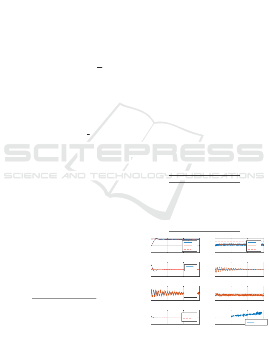
5.1 Regulation Task
The main goal is to solve a regulation problem, hav-
ing x
d
= 8[m] and z
d
= 3[m]. A first set of tests
are provided to show the performance of the system
without/with the disturbance compensation either in
Table 1: Simulation parameters.
Parameter value
m
r
0.5[Kg]
m
p
m
r
/4[Kg]
l
p
0.35[m]
I
r
0.177
I
m
m
p
l
2
p
the translational and rotational subsystem. In this re-
gard, an external disturbance is applied in the rota-
tional subsystem to observer the consequences when
the center of gravity shifts away.
• The behavior of the rotorcraft when the coupling
disturbance are not compensates is depicted on
Fig.3.
• The states behavior using the estimated distur-
bances is shown by Fig.4.
• Following a progressive criteria, now, let us show
the behavior of the rotorcraft, with and without
disturbance compensation, while a sudden torque
disturbance is exerted on the aerial pendulum at
t = 15[sec]. Such scenario is presented by Fig.5,
Fig.6
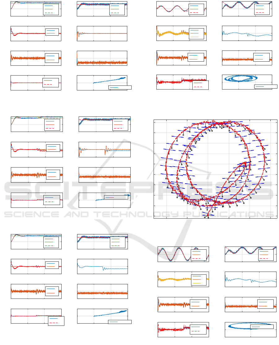
5.2 Trajectory Tracking Task
In this part of the paper, the commanded reference
is modified in order to appreciate the effectiveness of
the proposed approach while tracking a circular tra-
jectory x
d
(t) = 4 sin(2π f t) and z
d
(t) = 4 cos(2π f t).
The torque disturbance appearing at t = 15[sec] is still
considered. The behavior of the rotorcraft while fol-
lowing a trajectory without and with compensation is
displayed by Fig.7, Fig.8, Fig.9 and Fig.10
Table 2: Kalman Filter parameters. We have also added a
noise to sensor outputs whose variance value is R
i
= 1e−3.
Parameter value
T
samp
0.01[S]
Q
x
11
/Q
x
22
/Q
x
33
0/0/1
Q
z
11
/Q
z
22
/Q
z
33
0/0/1
Q
θ
11
/Q
θ
22
/Q
θ
33
0/0/1
l
p
0.35[m]
I
r
0.177
I
m
m
p
l
2
p
Time[sec]
0 10 20 30
x [m]
-10
0
10
x
x
est
x
d
Time[sec]
0 10 20 30
z[m]
-5
0
5
z
z
est
z
d
Time[sec]
0 10 20 30
3[deg]
-50
0
50
3
3
d
Time[sec]
0 10 20 30
.[deg]
-500
0
500
Time[sec]
0 10 20 30
;
x
-2
0
2
;
x
;
x
d
Time[sec]
0 10 20 30
;
z
-5
0
5
Time[sec]
0 10 20 30
;
3
-5
0
5
;
3
;
3
e
st
x[m]
-5 0 5 10
z[m]
-1
0
1
2D Motion
Figure 3: States evolution during a regulation task without
disturbance compensation.
Generalized Disturbance Estimation via ESLKF for the Motion Control of Rotorcraft Having a Rod-suspended Load
531

Time[sec]
0 10 20 30
x [m]
-10
0
10
x
x
est
x
d
Time[sec]
0 10 20 30
z[m]
-5
0
5
z
z
est
z
d
Time[sec]
0 10 20 30
3[deg]
-50
0
50
3
3
d
Time[sec]
0 10 20 30
.[deg]
-200
0
200
Time[sec]
0 10 20 30
;
x
-2
0
2
;
x
;
x
d
Time[sec]
0 10 20 30
;
z
-2
0
2
Time[sec]
0 10 20 30
;
3
-5
0
5
;
3
;
3
e
st
x[m]
-5 0 5 10
z[m]
-5
0
5
2D Motion
Figure 4: States evolution during a regulation task with dis-
turbance compensation.
Time[sec]
0 10 20 30
x [m]
-10
0
10
x
x
est
x
d
Time[sec]
0 10 20 30
z[m]
-5
0
5
z
z
est
z
d
Time[sec]
0 10 20 30
3[deg]
-50
0
50
3
3
d
Time[sec]
0 10 20 30
.[deg]
-200
0
200
Time[sec]
0 10 20 30
;
x
-2
0
2
;
x
;
x
d
Time[sec]
0 10 20 30
;
z
-5
0
5
Time[sec]
0 10 20 30
;
3
-5
0
5
;
3
;
3
e
st
x[m]
-5 0 5 10
z[m]
-5
0
5
2D Motion
Figure 5: States behavior without the disturbance compen-
sation in the rotational layer.
Time[sec]
0 10 20 30
x [m]
-10
0
10
x
x
est
x
d
Time[sec]
0 10 20 30
z[m]
-5
0
5
z
z
est
z
d
Time[sec]
0 10 20 30
3[deg]
-50
0
50
3
3
d
Time[sec]
0 10 20 30
.[deg]
-100
0
100
Time[sec]
0 10 20 30
;
x
-2
0
2
;
x
;
x
d
Time[sec]
0 10 20 30
;
z
-5
0
5
Time[sec]
0 10 20 30
;
3
-5
0
5
;
3
;
3
e
st
x[m]
-5 0 5 10
z[m]
-5
0
5
2D Motion
Figure 6: States behavior with the disturbance compensa-
tion in the rotational layer.
6 CONCLUDING REMARKS
The paper has presented a navigation strategy us-
ing a extended-state LKF-based disturbance estima-
Time[sec]
0 10 20 30
x [m]
-10
0
10
x
x
est
x
d
Time[sec]
0 10 20 30
z[m]
-10
0
10
z
z
est
z
d
Time[sec]
0 10 20 30
3[deg]
-50
0
50
3
3
est
3
d
Time[sec]
0 10 20 30
.[deg]
-100
0
100
Time[sec]
0 10 20 30
;
x
-2
0
2
;
x
;
xest
Time[sec]
0 10 20 30
;
z
-5
0
5
;
z
;
zest
Time[sec]
0 10 20 30
;
3
-1
0
1
;
3
;
3
e
st
x[m]
-5 0 5 10
z[m]
-10
0
10
2D Motion
Figure 7: States behavior without the disturbance compen-
sation in the rotational layer.
x[m]
-4 -2 0 2 4 6
z[m]
0
1
2
3
4
5
6
7
8
9
2D Motion
Figure 8: 2D motion without the disturbance compensation
in the rotational layer.
Time[sec]
0 10 20 30
x [m]
-5
0
5
x
x
est
x
d
Time[sec]
0 10 20 30
z[m]
-10
0
10
z
z
est
z
d
Time[sec]
0 10 20 30
3[deg]
-100
0
100
3
3
est
3
d
Time[sec]
0 10 20 30
.[deg]
-100
0
100
Time[sec]
0 10 20 30
;
x
-2
0
2
;
x
;
xest
Time[sec]
0 10 20 30
;
z
-5
0
5
;
z
;
zest
Time[sec]
0 10 20 30
;
3
-1
0
1
;
3
;
3
e
st
x[m]
-5 0 5
z[m]
-10
0
10
2D Motion
Figure 9: States behavior with the disturbance compensa-
tion in the rotational layer.
tion combined with a simple two-time scale control
scheme. Despite the time-scale separation between
dynamics, the structure of LKF is shared by the trans-
ICINCO 2016 - 13th International Conference on Informatics in Control, Automation and Robotics
532

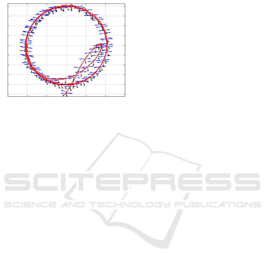
x[m]
-6 -4 -2 0 2 4 6
z[m]
0
1
2
3
4
5
6
7
8
9
2D Motion
Figure 10: 2D motion with the disturbance compensation in
the rotational layer.
lational and rotational dynamic layers, i.e. it uses the
same sampling time. The approach has show its ef-
fectiveness in two scenarios where the couplings has a
significant adverse effect on the overall performance,
either for a simple regulation or trajectory tracking
tasks. The modularity of the approach will allows to
extend the approach to the 3D case under windy con-
ditions.
REFERENCES
Bernard, M., Kondak, K., and Hommel, G. (2010). Load
transportation system based on autonomous small size
helicopters. Aeronautical Journal, 114(1153):191–
198.
Cruz, P. and Fierro, R. (2014). Autonomous lift of a
cable-suspended load by an unmanned aerial robot.
In 2014 IEEE Conference on Control Applications
(CCA), pages 802–807.
Faust, A., Palunko, I., Cruz, P., Fierro, R., and Tapia,
L. (2013). Learning swing-free trajectories for uavs
with a suspended load. In Robotics and Automa-
tion (ICRA), 2013 IEEE International Conference on,
pages 4902–4909.
Ghadiok, V., G. J. and Ren, W. On the design and devel-
opment of attitude stabilization, vision- based naviga-
tion, and aerial gripping for a low-cost quadrotor.
Ghadiok, V., G. J. and Ren, W. (2012). Autonomous
indoor aerial gripping using a quadrotor. In In
2011 IEEE/RSJ International Conference on Intelli-
gent Robots and Systems.
Kuntz, N. R. and Oh, P. Y. (2008). Towards autonomous
cargo deployment and retrieval by an unmanned aerial
vehicle using visual servoing. In ASME 2008 Interna-
tional Design Engineering Technical Conferences and
Computers and Information in Engineering Confer-
ence, pages 841–849. American Society of Mechan-
ical Engineers.
Mellinger, D., Shomin, M., and Kumar, V. (2010). Con-
trol of quadrotors for robust perching and landing. In
Proceedings of the International Powered Lift Confer-
ence, pages 205–225.
Palunko, I., Fierro, R., and Cruz, P. (2012). Trajectory
generation for swing-free maneuvers of a quadro-
tor with suspended payload: A dynamic program-
ming approach. In IEEE International Conference on
Robotics and Automation (ICRA) 2012, pages 2691–
2697.
Pizetta, I. H. B., Brando, A. S., and Sarcinelli-Filho, M.
(2015). Modelling and control of a pvtol quadro-
tor carrying a suspended load. In Unmanned Aircraft
Systems (ICUAS), 2015 International Conference on,
pages 444–450.
Pounds, P. E., Bersak, D., and Dollar, A. (2011). Grasping
from the air: Hovering capture and load stability. In
Robotics and Automation (ICRA), 2011 IEEE Interna-
tional Conference on, pages 2491–2498.
Thomas, J., Loianno, G., Sreenath, K., and Kumar, V.
(2014). Toward Image Based Visual Servoing for
Aerial Grasping and Perching. In ICRA. IEEE.
Yeol, J. W. and Lin, C.-H. (2014). Development of multi-
tentacle micro air vehicle. In Unmanned Aircraft
Systems (ICUAS), 2014 International Conference on,
pages 815–820.
Generalized Disturbance Estimation via ESLKF for the Motion Control of Rotorcraft Having a Rod-suspended Load
533