Dynamic Coupling Map: Acceleration Space Analysis for Underactuated
Robots
Ziad Zamzami and Faiz Ben Amar
Sorbonne Universites, UPMC Paris VI, Institut Syst`emes Intelligents et de Robotique,
ISIR - CNRS UMR 7222, Boite courrier 173, 4 Place JUSSIEU, 75252, Paris, France
Keywords:
Underactuated Robotics, Trajectory Optimization, Dynamic Coupling, Passive Dynamics, Acceleration
Space, Dynamic Capability Visualization.
Abstract:
Swing-up and throwing tasks for underactuated manipulators are examples of dynamic motions that exhibit
highly nonlinear coupling dynamics. One of the key ingredients for such complex behaviors is motion coordi-
nation to exploit their passive dynamics. Despite the existence of powerful tools such as nonlinear trajectory
optimization, they are usually treated as blackboxes that provide local optimal trajectories. We introduce the
Dynamical Coupling Map (DCM), a novel graphical technique, to help gain insight into the output trajectory
of the optimization and analyze the capability of underactuated robots. The DCM analysis is demonstrated
on the swing up motion of a simplified model of a gymnast on high bar. The DCM shows in a graphical
and intuitive way the pivotal role of exploiting the nonlinear inertial forces to reach the unstable equilibrium
configuration while taking into account the torque bounds constraints. In this paper, we present the DCM
as a posteriori analysis of a local optimal trajectory, found by employing the direct collocation trajectory
optimization framework.
1 INTRODUCTION
Humans and animals are capable of overcoming com-
plex terrain challenges with graceful and agile move-
ments. One of the key ingredients for such complex
behaviors is motion coordination to exploit natural
dynamics. Sports performers coordinate their action
in many different ways to achieve their goals. Coor-
dination is a key feature from the graceful, precise ac-
tion of an ice dancer to the explosive, physical power
of a triple jumper. Lizard coordinate its tail swing to
stabilize its dynamic motion over rough terrain (Libby
et al., 2012). Cheetah can rapidly accelerate and ma-
neuver during the pursuit of its prey by the coordinat-
ing of the motion of its tail (Patel and Braae, 2013).
Understanding and emulating these motions is the one
of the long-standing grand challenges in robotics and
biomechanics,with possible applications in rehabili-
tation, sport, search-and-rescue, environmental moni-
toring and security.
Unlike conventional fully-actuated manipulators
where the natural dynamics can be suppressed by
classical feedback control techniques, a large and di-
verse array of dynamical systems falls under the class
of underactuated systems. The unactuated nature
gives rise to many interesting control problems which
require fundamental non-linear approaches (Spong,
1998). Underactuated systems are defined as mechan-
ical systems in which the dimension of the configu-
ration space exceeds that of the control input space,
i.e. fewer control inputs than the available degrees of
freedom. Such restriction can be the result of 1)an ac-
tuator failure (Arai et al., 1998); 2) intentional choice
of a minimalist design which leads to a less costly,
lighter and more compact machine; 3) rigid robots
with elastic joints or flexible links (Spong, 1998); 4)
or even imposed by the nature of the system itself
such as non-prehensile manipulation (Lynch and Ma-
son, 1996) and recently extended to legged robots as
floating base systems (Wieber Pierre-Brice, Tedrake
Russ, 2015).
Synthesizing motion behavior for such underac-
tuated systems is quite challenging. Underactuation
impose constraints on their dynamics that restrict the
family of trajectories their configurations and acceler-
ations can follow. These constraints are second-order
nonholonomic constraints (Wieber, 2005)(Nagarajan
et al., 2013). Moreover, cannot be fully feedback
linearized (Spong, 1995). Underacuated system can
only be controlled indirectly either through contact
forces with the environment or through inertial forces
which rises from the nonlinear inertial coupling of the
548
Zamzami, Z. and Amar, F.
Dynamic Coupling Map: Acceleration Space Analysis for Underactuated Robots.
DOI: 10.5220/0006012405480557
In Proceedings of the 13th International Conference on Informatics in Control, Automation and Robotics (ICINCO 2016) - Volume 2, pages 548-557
ISBN: 978-989-758-198-4
Copyright
c
 2016 by SCITEPRESS – Science and Technology Publications, Lda. All rights reserved

articulated system (Tamegaya et al., 2008), in this pa-
per we focus on the latter.
(Hauser and Murray, 1990) introduced a canoni-
cal model of underactuated systems known as the Ac-
robot (for acrobatic robot) introduced by (Hauser and
Murray, 1990). It can be considered is a highly sim-
plified model of a human gymnast on the high bar,
where the underactuated first joint models the gym-
nast’s hands on the bar, and the actuated second joint
models the gymnast’s hips. The objective is to swing
up the Acrobot from the downward stable equilib-
rium point to the upright unstable equilibrium point
and balance it about the upright vertical. This motion
control problem is usually decomposed into two sub-
problems; first, the swing-up motion control (
˚
Astr¨om
and Furuta, 2000) (Spong, 1995) (Xin, 2013), once
the robot’s configuration is brought up to the neigh-
borhood of the unstable equilibrium point, switching
to a stabilization controller is necessary(Olfati-Saber,
2001). Several variants of the Acrobot have been pro-
posed either increasing the number of degrees of free-
doms (Kurazume and Hasegawa, 2002) (Shkolnik and
Tedrake, 2008) (Ibuki et al., 2015) or by varying the
placement of the actuators (Luca and Oriolo, 2002).
For the sake of illustration, we focus in this paper,
on an extended version of the acrobat called the gym-
nast introduced by (Xin and Kaneda, 2007b) arguing
the importance of a third active joint representing the
shoulder.
During the last two decades, many researchers
have investigated the approach of passivity or energy-
based control of underactuated mechanical systems.
(Lam and Davison, 2006) showed that the coupling
becomes more complex when the number of links
increases, and its control problem becomes more
challenging. (Xin and Kaneda, 2007a) noted that
energy based techniques are difficult to apply for
higher dimension robots.
1.1 Approach and Contribution
In this work, we employ nonlinear trajectory opti-
mization for the swing-up motion generation and con-
trol. Second-order Nonholonomic and torque con-
straints fit naturally into the direct formulation of tra-
jectory optimization. Furthermore, there exists strong
evidence that humans solve task-level and motor-level
challenges though optimization processes. A good
overview of optimal control in sensorimotor systems
is given by (Todorov, 2004).
Trajectory optimization approach is becoming in-
creasingly attractive with the advent of computational
power and the recent advances in nonlinear optimiza-
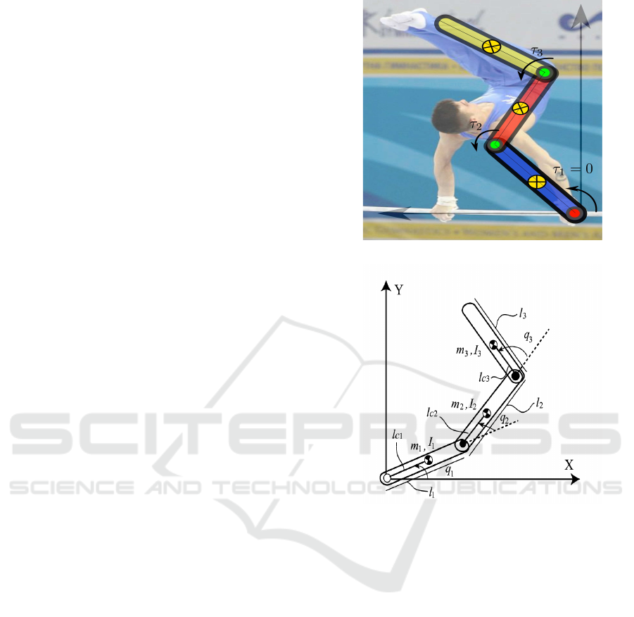
Figure 1: Simplified model of a gymnast on a high bar.
Figure 2: 3-link Gymnast model of underactuated mechan-
ical system with passive joint at the base.
tion (Posa et al., 2013)(Hauser, 2014). Given an ini-
tial trajectory that may be non-optimal or even non-
feasible, trajectory optimization methods can often
quickly converge to a high-quality, locally-optimal
solution.
We analyze the output trajectory using a novel
graphical technique that we call ”Dynamic Coupling
Map (DCM)” that help gain insight into the motion
of the system. Our ultimate goal for studying such
systems is to understand problems of dynamic loco-
motion in both biological systems and in robotic sys-
tems.
The rest of the paper is structured as follow. Sec-
tion (2) describes the Lagrangian dynamics of under-
actuated mechanical systems. A presentation of the
trajectory optimization formulation is given in section
(3). In section (4), we derive the dynamic coupling el-
lipsoid in both the unactuated acceleration space and
the task space. The results of the numerical simula-
tion and a discussion on the benefits of the Dynamic
Dynamic Coupling Map: Acceleration Space Analysis for Underactuated Robots
549

Coupling Map as a graphical analysis tool to gain in-
sight to the full acceleration capabilities of the under-
actuated system is given in(5). A discussion on possi-
ble extensions completes the paper.
2 LANGRANGIAN DYNAMICS
OF UNDERACTUATED
MECHANICAL SYSTEMS
Consider a dynamic system defined on a configuration
manifold Q . let (q, ˙q) = (q
1
,. .. ,q
n
, ˙q
1
,. .. , ˙q
n
) denote
local coordinates on the tangent bundle T Q . We refer
to q, ˙q, and ¨q as the vectors of generalized coordinates,
generalized velocities, and generalized accelerations,
respectively. Let the system possess a control input
space of dimension m < n, where u ∈ R
m
denote the
vector of the control variables. Without loss of gen-
erality, we decompose the set of generalized coordi-
nates q = (q
1
,. .. ,q
n
) ∈ R
n
into q = (q
p
,q
a
) where
q
p
∈ R
n−m
, q
a
∈ R
m
denote the passive degrees of
freedom and the actuated degrees of freedom.
q =

q
p
(n−m×1)
q
a
(m×1)

∈ ℜ
n
(1)
We can then write the Euler-Lagrange equation of
motion in a canonical form as

M
pp
M
pa
M
T
pa
M
aa

¨q
p
¨q
a

+

N
p
(q, ˙q)
N
a
(q, ˙q)

=

0
τ

(2)
where the joint space inertia matrix is decomposed
into:
• M
pp
: represents The inertia matrix for the system
seen at the passive articulating subsystem
• M
aa
: represents The inertia matrix of the active
articulating subsystem
• M
pa
: The inertial coupling term between the ac-
tive and passive articulating subsystems
• ¨q
p
is the second derivative of the floating base’s
pose (position and orientation) w.r.t time. While
¨q
q
is the m-actuated joints acceleration.
• τ: The vector of the joint torques of the articulated
system, assuming that articulated system is fully
actuated.
• N
a
(q, ˙q): is the generalized bias force, it follows
that it is the value that τ would have to take in
order to produce zero joint acceleration, assum-
ing that all the other joint accelerations are zero.
Generalized bias force is a vector of force terms
that account for Coriolis and centrifugal forces,
gravity. We assume that there exist no external
wrenches, for the sake of the clarity of presenta-
tion.
• N
p
(q, ˙q): is the generalized bias force acting on
the passive subsystem.
3 TRAJECTORY OPTIMIZATION
A trajectory optimization problem seeks to find the
a trajectory for some dynamical system that satisfies
some set of equality and inequality constraints con-
straints while minimizing some cost functional.
An abstraction of the Lagrangian dynamics in Eq.(2)
can be written as a set of differential equations
˙x(t) = f(x(t),u(t)) (3)
where x =

q
˙q

∈ R
2n
represent the system states, as-
suming the number of generalized coordinates equal
to the number of generalized velocities. The input
control vector u ∈R
m
and the transition function f()
defines the system evolution in time. Trajectory op-
timization problem seeks to find a finite-time input
trajectory u(t),∀ ∈ [0,t
f
], such that a given criteria is
minimized,
G = φ(t
0
,x
0
,t
f
,x
f
) +
t
f
Z
t
0
g(t, x, u) dt (4)
where φ() and g() are the intermediate and final
cost function. The objectivefunction can be written in
terms of quantities evaluated at the ends of the phases
only, in that case it is referred to as the Mayer form.
If the objective function only involves an integral it is
referred to as a problem of Lagrange, and when both
terms are present it is called a problem of Bolza.
The optimization may be subject to a set of bound-
ary constraints
b
min
< b(t
0
,x
0
) < b
max
(5)
b
min
< b(t
f
,x
f
) < b
max
(6)
In addition, Dynamic constraints, including the sec-
ond order non-holonomic constraints, can be added
as path constraints
c
min
< c(t, x(t), u(t)) < c
max
(7)
Bounds on state variables and input control limits are
added as
x
min
≤ x(t) ≤ x
max
(8)
u
min
≤ u(t) ≤ u
max
(9)
The result of the optimization is an optimal trajec-
tory given by [x
∗
(t),u
∗
(t)]
ICINCO 2016 - 13th International Conference on Informatics in Control, Automation and Robotics
550

To compute a feasible motion plan we transcribe
the differential equation of the robot dynamics to al-
gebraic equations and solve them through NonLinear
Optimisation (NLP). (Betts, 2010) showed that that
NLP can be interpreted as discrete approximations of
the continuous optimal control problem. There are
mature NLP solvers used in robotics; SNOPT (Gill
et al., 2002) which is based on Sequential Quadratic
Programming (SQP). The second solver is iPOPT
(Wachter and Biegler, 2006) using the Interior Point
Method. However, The complete description of the
solvers and the algorithms used lies outside of the
scope of this paper.
We employ direct method for transcribing and
solving the optimal control problem. The solution to
an optimal control problem via direct methods scales
well to high-dimensional systems. In direct collo-
cation, the optimization searches over a set of deci-
sion variables z, comprised by a vector of the states
and control trajectories discretized over time at cer-
tain points or nodes, i.e., z = [xk, uk], for k = 1,...,N,
where N represents the total number of nodes. Finally
The NLP can be formulated as.
minimize
z
G(z) (10)
subject to : l ≤


z
c(z)
Az


≤ u (11)
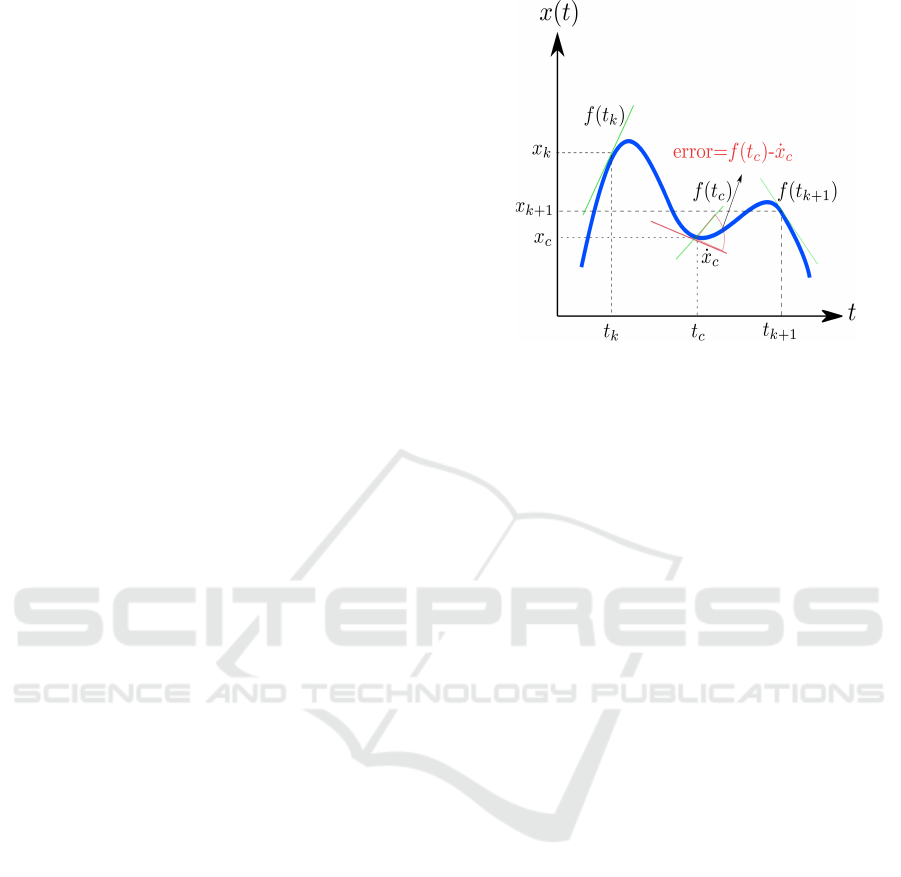
In, direct collocation the input is represented as a
piecewise-linear. function of time, and the state is
piecewise-cubic. The values of the state and con-
trol at each knot point are the decision variables.
The slope of state is prescribed by the dynamics at
each knot point. The collocation points are the mid-
vpoints of each cubic segment. The slope of the cu-
bic at the collocation point is constrained to match
the system dynamics at that point, as illustrated in
figure(3). For more details the reader is referred to
(Betts, 2010)(Betts, 1998).
4 DYNAMIC COUPLING MAP
4.1 Dynamic Coupling in the
Unactuated Acceleration Space
Kinematic and dynamic coupling between the articu-
lated system and the base is usually regarded as un-
wanted perturbation that degrades positioning accu-
racy and operational dexterity. In this work we at-
tempt to exploit the dynamic coupling between the
unactuated subsystem and its associated active artic-
ulated subsystem. we will start first by exploring the
Figure 3: Illustration of the state trajectory discretization
occurring in direct collocation optimization. System dy-
namics f (t
c
) are enforced to match the slope of the cubic
˙x
c
at the collocation point x
c
.
relationship between the acceleration space of the un-
actuated subsystem and the torque space of the active
articulating subsystem.
The dynamic equations of the system (2) can be de-
composed into two main equations; one describing
the dynamics of the passive free-floating base.
M
p
¨q
p
+ M
pa
¨q
a
+ N
p
= 0 (12)
and the second equation describing the dynamics
of the articulated system
M
a
¨q
a
+ M
T
pa
¨q
p
+ N
a
= τ (13)
For the sake of clarity, we dropped the dependence of
the force bias terms N
a,p
on q, ˙q.
Definition 4.1. The underactuated mechanical
system (2) is locally Strongly Inertially Coupled if
and only if
rank(M
bm
(q)) = n −m forall q ∈ B
where B is a neighborhood of the origin. The
Strong Inertial Coupling is global if the rank condi-
tion holds for all q ∈Q
the strong inertial coupling condition (Spong,
1998) requires that the number of active degrees of
freedom be at least as great as the number of passive
degrees of freedom.
Under the assumption of Strong Inertial Coupling we
may compute a pseudo-inverse M
†
pa
for M
pa
as
M
†
pa
= M
T
pa
(M
pa
M
T
pa
)
−1
(14)
Then active joints generalized accelerations
¨
ˆq in
(12) can be expressed as
¨q
a
= −M
†
pa
M
p
¨q
p
−M
†
pa
N
p
(15)
Dynamic Coupling Map: Acceleration Space Analysis for Underactuated Robots
551

By substituting (15) in (13), we can find a relation
between the acceleration of the passive subsystem and
its acting surrounding, which include; Joint torques,
Nonlinear inertial forces, Gravity and wrench acting
on the end points of the articulated system, if exists.
¨q
p

M
T
pa
−M
a
M
†
pa
M
p

−M
a
M
†
pa
N
p
+ N
a
= τ (16)
we finally express equation (16) as
¨q
p
= Z
†

τ+
f
N

= ¨q
p
τ
+ ¨q
p
bias
(17)
where we introduce the dynamic coupling factor Z
†
as
Z
†
=

M
T
pa
−M
a
M
†
pa
M
p

†
(18)
Z is the Schur complement (Kolda and Bader, 2008)
of the inertia coupling M
bq
between the passive sub-
system and the active articulating system We denote,
as well, the bias term.
f
N = M
a
M
†
pa
N
p
−N
a
(19)
equation (17) provides an intuitive comprehension of
the influence of different forces on the motion of the
passive subsytem: ¨q
p
τ
is the acceleration of the pas-
sive subsystem due to the torques of the active artic-
ulated system, ¨q
p
bias
is the acceleration due to gravity
and non-linear inertial forces, and wrenches acting on
the articulated system such as contact forces.
Furthermore, we note that the inverse of the dy-
namic coupling factor Z
†
act as transmission factor
between the control input space τ and the acceleration
space of the passive subsystem. Z
†
is configuration-
dependent matrix. Thereby, it is possible to search
for the configurationthat maximizes the dynamiccou-
pling factor which will result in a decrease in the ef-
fort expenditure. This formulation of the dynamic
equation helps in analyzing the effects of these three
sets of variables on the achievable set of free floating
base acceleration.
4.2 Dynamic Coupling Ellipsoid
The goal of the Floating base dynamic coupling ellip-
soid is to represent geometrically, in the acceleration
space, the ensemble of the accelerations achievable by
the unactuated subsystem. The torque limits at each
actuator in the articulated system are assumed to be
symmetrical, that is,
−τ
i,max
≤τ
i
≤ τ
i,max
(20)
The normalized joint torque vector
˜
τ can be expressed
as
˜
τ = L
−1
τ (21)
where the scaling matrix L is given by
L = diag(τ
1,max
,τ
2,max
,. . . ,τ
n,max
) (22)
The control input space can then be represented as m-
dimensional sphere defined by
˜
τ
T
˜
τ ≤ 1 (23)
By solving Eq.(17) and substituting in Eq.(23) we get
the equation of an ellipsoid in the acceleration space
of the passive subsystem.
( ¨q
p
− ¨q
p
bias
)
T
(Z
†
L)
−T
(Z
†
L)
−1
( ¨q
p
− ¨q
p
bias
)
T
≤ 1
(24)
which simplifies to
( ¨q
p
− ¨q
p
bias
)
T
˜
Z( ¨q
p
− ¨q
p
bias
)
T
≤ 1 (25)
where
˜
Z = Z
T
L
−2
Z (26)
By applying singular value decomposition,
˜
Z can
be decomposed into
˜
Z = U ΣV
T
(27)
where U ∈ R
m×m
and V ∈ R
n×n
are orthogonal ma-
trices. The principal axis of the n−m-dimensional
ellipsoid is determined by the eigenvectors u
i
, while
its length is specified by the corresponding eigenvalue
√
σ
i
. Furthermore, the term ¨q
bias
is responsible for
translating the ellipsoid center from its origin.
4.3 Dynamic Coupling in the Task
Space
In certain applications, it is more natural to reason
about the underactuated mechanical system in the
task space acceleration space, when it is more rel-
evant than the generalized accelerations space. We
extend the previous analysis to describe the dynamic
coupling between the active subsystem and the task
space, while taking into consideration the unactuated
nature of the mechanical system.
let X =

x
1
x
2
.. . x
d

T
denote the d-
dimensional task vector, which can represent the
Cartesian position of the end effector of the manip-
ulator or the center of mass of the underactuated sys-
tem or any configuration dependent task can be for-
mulated as X = f(q). By taking the Taylor expansion
of this mapping we derive the Jacobian that maps the
task space velocities to the generalized velocities of
the underactuated system.
˙
X = J(q) ˙q (28)
The task space acceleration can be found by differen-
tiating Eq.(28) with respect to time yielding
¨
X = J(q) ¨q+
˙
J(q, ˙q) ˙q (29)
ICINCO 2016 - 13th International Conference on Informatics in Control, Automation and Robotics
552

we partition further Eq.(29) into passive and active
subsystems as follows
¨
X = J
p
¨q
p
+ J
a
¨q
a
+
˙
J(q, ˙q) ˙q (30)
From Eq.(13) we can express the generalized acceler-
ation of the active subsystem function in torque as
¨q
a
=
¯
Z(τ −N
a
) (31)
where
¯
Z = M
T
pa
−M
aa
M
−1
pp
M
pa
(32)
The generalized acceleration of the passive subsystem
can also be expressed as
¨q
p
= −M
−1
pp
M
pa
¨q
a
−M
−1
pp
N
p
(33)
By substituting Eq.(31) in Eq.(33) we get
¨q
p
= −M
−1
pp
M
pa
(
¯
Z(τ−N
a
)) −M
−1
pp
N
p
(34)
To find the relationship between the Task space ac-
celeration to the control input space, we substitute
Eq.(34) and Eq.(31) in Eq.(29)
¨
X = Z
∗
τ+
¨
X
bias
(35)
where Z
∗
and
¨
X
bias
are defined as
Z
∗
= J
a
¯
Z −J
p
M
−1
pp
M
pa
¯
Z (36)
¨
X
bias
= J
p
M
−1
pp
M
pa
N
p
−J
p
M
−1
pp
N
a
−J
a
¯
ZN
a
+
˙
J(q, ˙q) ˙q
(37)
Following the same procedure in 4.2 for deriving the
dynamic coupling ellipsoid in the generalized accel-
eration space , we can define the dynamic coupling
ellipsoid in the task space
(
¨
X −
¨
X
bias
)
T
(Z
∗
L)
−T
(Z
∗
L)
−1
(
¨
X −
¨
X
bias
) ≤ 1 (38)
5 EXPERIMENT RESULTS
5.1 Model Description
For the purpose of illustration, we focus our atten-
tion to the swing-up dynamic motion of the ’Gym-
nast’ robot shown in figure (2). The Gymnast is a
highly simplified approximation of an athlete swing-
ing his body on a high bar. The model is composed
of 3 links representing the arm, the trunk and the leg.
All 3 links are connected by 1-DoF rotary joints. The
arm is connected to the world through a passive joint,
while the second and the third joint are active and
torque controlled. Assuming symmetrical motion, we
restrict our attention to the sagittal plane.
The inertial parameters used are; m
1
= 1 Kg, m
2
=
m
3
= 2 Kg denoting the masses of the first, second and
third link, respectively. The first link has a length of
l
1
= 1m while the second and third links have lengths
of l
2
= l
3
= 2m. Density assumed to be homogeneous,
thus l
c
1
= 0.5m and l
c
2
= l
c
3
= 1m denotes the relative
positions of the center of mass. The torque limits for
actuators are given by L = diag(10 N.m,10 N.m)
The robot is modeled using MIT toolbox Drake
(Tedrake, 2014) in a Matlab environment. The
optimization problem is solved using a non-linear
optimization solver SNOPT based on Sequential
Quadratic Program (SQP) algorithm.
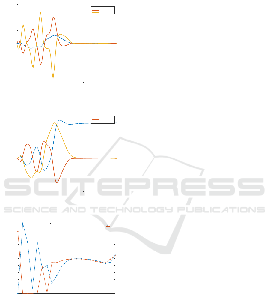
5.2 Results
The non-linear optimization solver finds a local-
optimal trajectory for the dynamic swing up motion
of the Gymnast robot. Figure (4) shows a compila-
tion of the motion from the down equilibrium position
q =

q
1
q
2
q
3

T
=

0 0 0

T
to the up-right un-
stable equilibrium position q =

π 0 0

T
. The first
link is shown in blue, while the second and third links
are shown in red and yellow, respectively. Figure (6)
and figure (5) shows the evolution of the generalized
position and velocities during swing up motion, re-
spectively. We can note that although we have set an
initial guess of the time span of the motion to be t
0
= 6
seconds the optimization achieved the goal configura-
tion with an optimal time of t
∗
≃ 4. Figure (7) shows
the optimal torque control policy for the actuated sub-
system, τ
2
& τ
3
in this case.
The Dynamic coupling analysis is depicted in
Table(1), Table (2) & Table (3). Each column repre-
sents an instance of the motion with an interval of 0.3
seconds. The first row shows snapshots of the config-
urations of the ’Gymnast’ robot during the swing-up
trajectory. The second row shows only the shape of
the corresponding dynamic coupling ellipsoids in the
task space. In this case, it offers an intuitive Carte-
sian acceleration of the terminal organ representing
the foot (colored in purple). The horizontal acceler-
ation is depicted on the abscissa, while the vertical
acceleration is depicted on the ordinate. The prin-
cipal axis and scale of the dynamic coupling ellip-
soid is determined by singular value decomposition
of (Z
∗
L)
−T
(Z
∗
L)
−1
in equation (38). The third row
shows the trajectory of the dynamic coupling ellipsoid
while taking into consideration the non-linear inertial
forces. Unlike row 2 which shows the dynamic cou-
pling ellipsoid centered at the origin, row 3 shows the
displaced ellipsoid due to the contribution of the non-
linear inertial forces
¨
X
bias
in equation (37). The vector
of displacement from the instantaneous origin is rep-
resented by an arrow.
Dynamic Coupling Map: Acceleration Space Analysis for Underactuated Robots
553

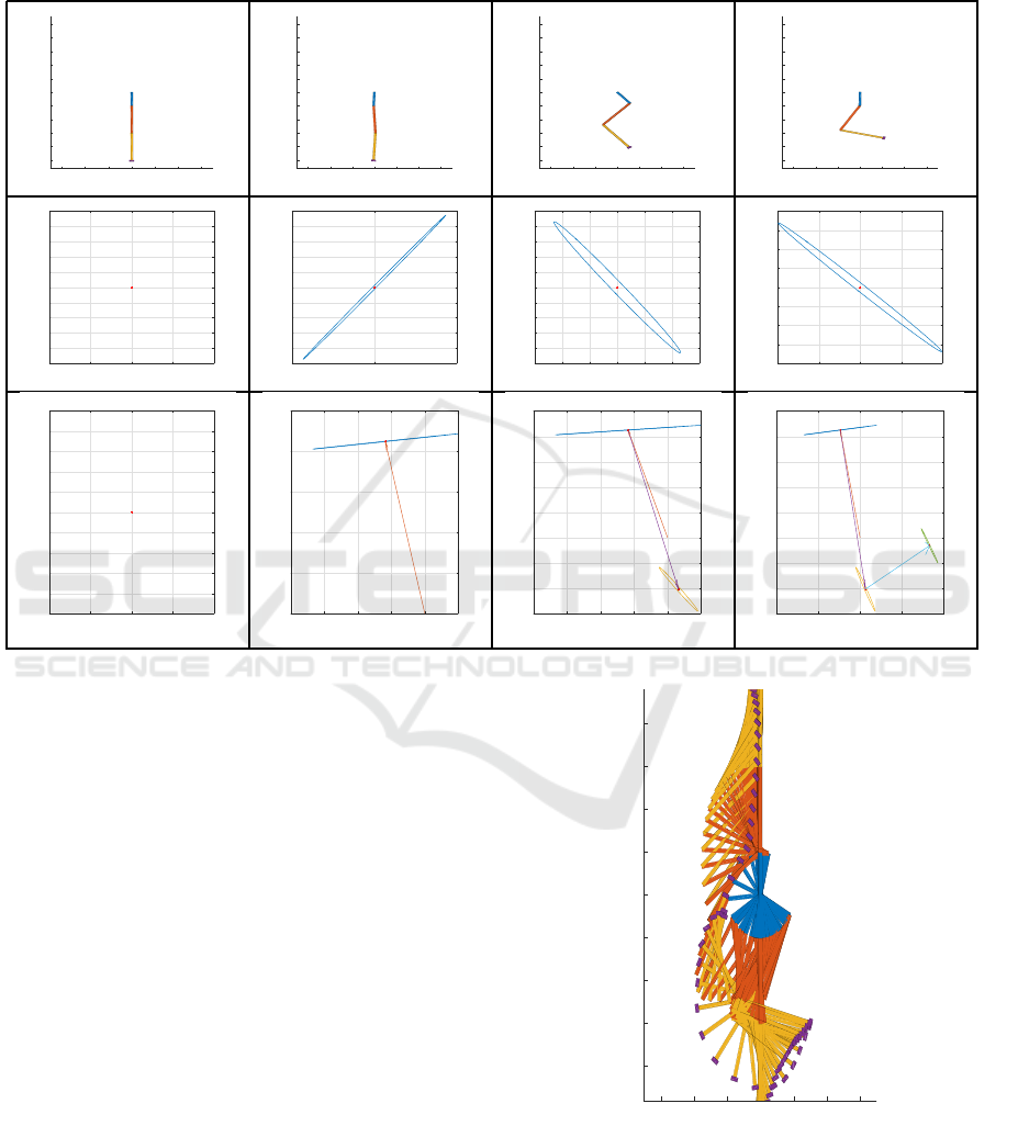
Table 1: Snapshots of the swing-up trajectory: The first row shows the configurations of the ’Gymnast’ robot during the
swing-up trajectory. The second row shows the shape of corresponding dynamic coupling ellipsoids. The Third row shows
the trajectory of the dynamic coupling ellipsoid while taking into consideration the non-linear inertial forces. The first link
with a passive joint is shown in blue. The second and third link with active joints are shown in red and yellow, rescpectively.
-3 -2 -1 0 1 2 3
x
-5
-4
-3
-2
-1
0
1
2
3
4
5
z
t = 0.00 sec
-3 -2 -1 0 1 2 3
x
-5
-4
-3
-2
-1
0
1
2
3
4
5
z
t = 0.30 sec
-3 -2 -1 0 1 2 3
x
-5
-4
-3
-2
-1
0
1
2
3
4
5
z
t = 0.60 sec
-3 -2 -1 0 1 2 3
x
-5
-4
-3
-2
-1
0
1
2
3
4
5
z
t = 0.90 sec
-1 -0.5 0 0.5 1
Horizontal acceleration (m/s
2
)
-1
-0.8
-0.6
-0.4
-0.2
0
0.2
0.4
0.6
0.8
1
Vertical acceleration (m/s
2
)
Dynamic Coupling Ellipsoid
-50 0 50
Horizontal acceleration (m/s
2
)
-1
-0.8
-0.6
-0.4
-0.2
0
0.2
0.4
0.6
0.8
1
Vertical acceleration (m/s
2
)
Dynamic Coupling Ellipsoid
-15 -10 -5 0 5 10 15
Horizontal acceleration (m/s
2
)
-5
-4
-3
-2
-1
0
1
2
3
4
5
Vertical acceleration (m/s
2
)
Dynamic Coupling Ellipsoid
-10 -5 0 5 10
Horizontal acceleration (m/s
2
)
-4
-3
-2
-1
0
1
2
3
4
Vertical acceleration (m/s
2
)
Dynamic Coupling Ellipsoid
-1 -0.5 0 0.5 1
Horizontal acceleration (m/s
2
)
-1
-0.8
-0.6
-0.4
-0.2
0
0.2
0.4
0.6
0.8
1
Vertical acceleration (m/s
2
)
Dynamic Coupling Ellipsoid
-80 -60 -40 -20 0 20
Horizontal acceleration (m/s
2
)
0
5
10
15
20
25
Vertical acceleration (m/s
2
)
Dynamic Coupling Map
-80 -60 -40 -20 0 20
Horizontal acceleration (m/s
2
)
-15
-10
-5
0
5
10
15
20
25
Vertical acceleration (m/s
2
)
Dynamic Coupling Map
-100 -50 0 50 100
Horizontal acceleration (m/s
2
)
-15
-10
-5
0
5
10
15
20
25
Vertical acceleration (m/s
2
)
Dynamic Coupling Map
5.3 Discussion
Trajectory optimization proved to be an interesting
approach to generate high quality dynamic motion de-
spite its local optimality aspect. Moreover, its natu-
ral capacity to integrate all types of constraints (lin-
ear, nonlinear, complementarity problems), objective
functions and application-related heuristics allowed it
to gain traction in the robotics community. However,
after many iterations, the optimization solver outputs
a single local optimal trajectory without any insight
into the nature of the given trajectory. The swing up
motion example illustrates the emergence of nontriv-
ial solution to the torque control, velocity and position
trajectory from simple core principles (goal configu-
ration, torque limit, dynamic model).
We use the Dynamic Coupling map (DCM) to an-
alyze the dynamic motion given by the optimization.
To facilitate the navigation and explanation of the
DCM, let the location of each cell in table (1) be given
by the triplet (t,r, c), where t r and c corresponds to
the number of table, row and column, respectively.
The ’Gymnast’ starts from an equilibrium position de-
picted in cell(1,1,1), where the dynamic coupling el-
-3 -2 -1 0 1 2 3
x
-4
-3
-2
-1
0
1
2
3
4
z
t = 6.00 sec
Figure 4: Local-optimal swing-up motion.
lipsoid in the task space representing the maximum
acceleration capacity of the terminal organ (shown
in purple) is shown in cell(1,2,1). Since the starting
configuration is singular the Jacobian-dependent el-
ICINCO 2016 - 13th International Conference on Informatics in Control, Automation and Robotics
554

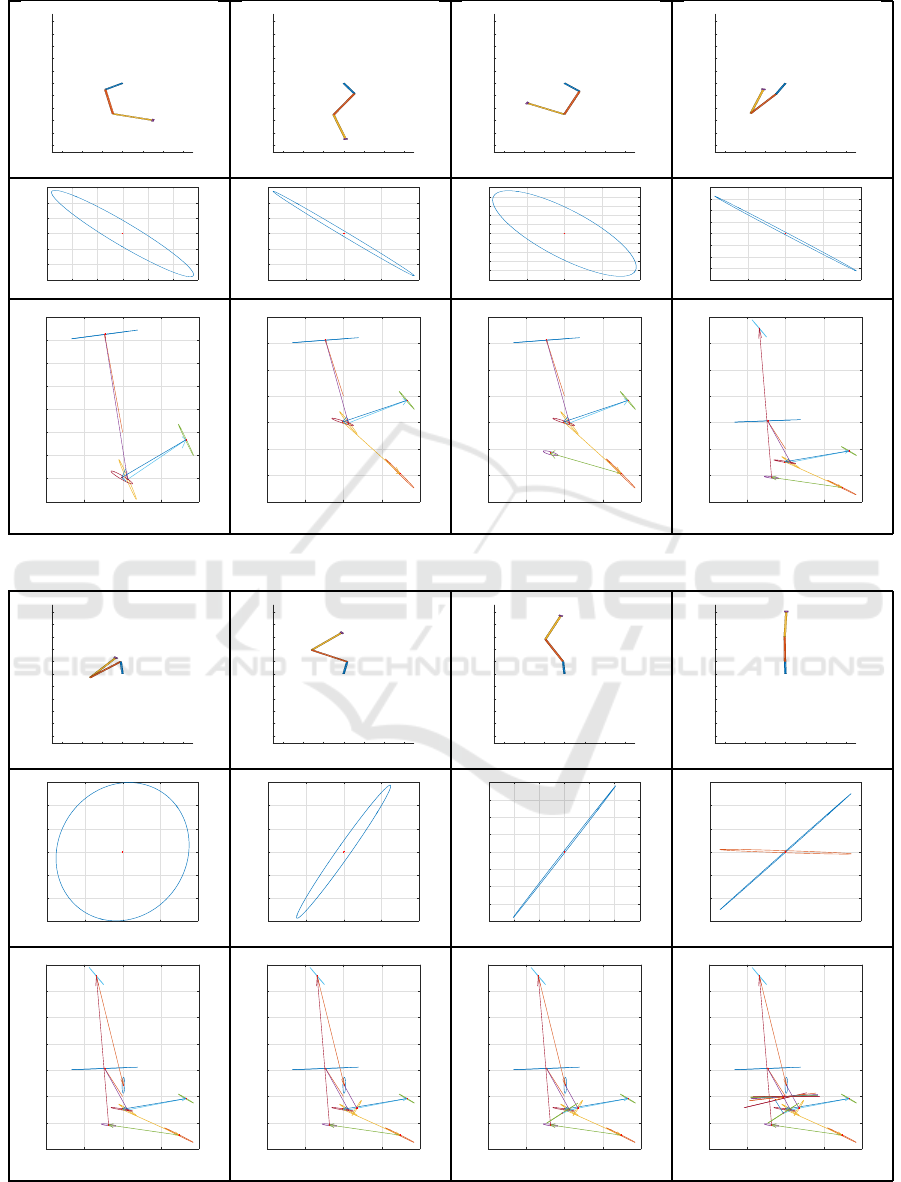
Table 2: Continued.
-3 -2 -1 0 1 2 3
x
-5
-4
-3
-2
-1
0
1
2
3
4
5
z
t = 1.20 sec
-3 -2 -1 0 1 2 3
x
-5
-4
-3
-2
-1
0
1
2
3
4
5
z
t = 1.50 sec
-3 -2 -1 0 1 2 3
x
-5
-4
-3
-2
-1
0
1
2
3
4
5
z
t = 1.80 sec
-3 -2 -1 0 1 2 3
x
-5
-4
-3
-2
-1
0
1
2
3
4
5
z
t = 2.10 sec
-15 -10 -5 0 5 10 15
Horizontal acceleration (m/s
2
)
-1.5
-1
-0.5
0
0.5
1
1.5
Vertical acceleration (m/s
2
)
Dynamic Coupling Ellipsoid
-20 -10 0 10 20
Horizontal acceleration (m/s
2
)
-6
-4
-2
0
2
4
6
Vertical acceleration (m/s
2
)
Dynamic Coupling Ellipsoid
-10 -5 0 5 10
Horizontal acceleration (m/s
2
)
-1
-0.8
-0.6
-0.4
-0.2
0
0.2
0.4
0.6
0.8
1
Vertical acceleration (m/s
2
)
Dynamic Coupling Ellipsoid
-10 -5 0 5 10
Horizontal acceleration (m/s
2
)
-8
-6
-4
-2
0
2
4
6
8
Vertical acceleration (m/s
2
)
Dynamic Coupling Ellipsoid
-100 -50 0 50 100
Horizontal acceleration (m/s
2
)
-15
-10
-5
0
5
10
15
20
25
Vertical acceleration (m/s
2
)
Dynamic Coupling Map
-100 -50 0 50 100
Horizontal acceleration (m/s
2
)
-40
-30
-20
-10
0
10
20
30
Vertical acceleration (m/s
2
)
Dynamic Coupling Map
-100 -50 0 50 100
Horizontal acceleration (m/s
2
)
-40
-30
-20
-10
0
10
20
30
Vertical acceleration (m/s
2
)
Dynamic Coupling Map
-100 -50 0 50 100
Horizontal acceleration (m/s
2
)
-40
-20
0
20
40
60
80
100
Vertical acceleration (m/s
2
)
Dynamic Coupling Map
Table 3: Continued.
-3 -2 -1 0 1 2 3
x
-5
-4
-3
-2
-1
0
1
2
3
4
5
z
t = 2.40 sec
-3 -2 -1 0 1 2 3
x
-5
-4
-3
-2
-1
0
1
2
3
4
5
z
t = 2.70 sec
-3 -2 -1 0 1 2 3
x
-5
-4
-3
-2
-1
0
1
2
3
4
5
z
t = 3.00 sec
-3 -2 -1 0 1 2 3
x
-5
-4
-3
-2
-1
0
1
2
3
4
5
z
t = 5.10 sec
-2 -1 0 1 2
Horizontal acceleration (m/s
2
)
-6
-4
-2
0
2
4
6
Vertical acceleration (m/s
2
)
Dynamic Coupling Ellipsoid
-10 -5 0 5 10
Horizontal acceleration (m/s
2
)
-6
-4
-2
0
2
4
6
Vertical acceleration (m/s
2
)
Dynamic Coupling Ellipsoid
-30 -20 -10 0 10 20 30
Horizontal acceleration (m/s
2
)
-8
-6
-4
-2
0
2
4
6
8
Vertical acceleration (m/s
2
)
Dynamic Coupling Ellipsoid
-50 0 50
Horizontal acceleration (m/s
2
)
-0.6
-0.4
-0.2
0
0.2
0.4
0.6
Vertical acceleration (m/s
2
)
Dynamic Coupling Ellipsoid
-100 -50 0 50 100
Horizontal acceleration (m/s
2
)
-40
-20
0
20
40
60
80
100
Vertical acceleration (m/s
2
)
Dynamic Coupling Map
-100 -50 0 50 100
Horizontal acceleration (m/s
2
)
-40
-20
0
20
40
60
80
100
Vertical acceleration (m/s
2
)
Dynamic Coupling Map
-100 -50 0 50 100
Horizontal acceleration (m/s
2
)
-40
-20
0
20
40
60
80
100
Vertical acceleration (m/s
2
)
Dynamic Coupling Map
-100 -50 0 50 100
Horizontal acceleration (m/s
2
)
-40
-20
0
20
40
60
80
100
Vertical acceleration (m/s
2
)
Dynamic Coupling Map
Dynamic Coupling Map: Acceleration Space Analysis for Underactuated Robots
555

0 1 2 3 4 5 6
T ime(s)
-15
-10
-5
0
5
10
15
˙q (rad/s)
Generalized Velocity Profile
Passive Joint 1
Active Joint 2
Active Joint 3
Figure 5: Local-optimal Generalized Velocities Profile for
the swing-up motion.
0 1 2 3 4 5 6
T ime(s)
-3
-2
-1
0
1
2
3
4
q (rad)
Generalized Configuration Profile
Passive Joint 1
Active Joint 2
Active Joint 3
Figure 6: Local-optimal Generalized Coordinates Profile
for the swing-up motion.
0 1 2 3 4 5 6
T ime(s)
-10
-8
-6
-4
-2
0
2
4
6
8
10
T orque(N .m)
Joint Effort Profile
Joint 2
Joint 3
Figure 7: Local-optimal Torque Control Profile for the
swing-up motion.
lipsoid fails to give any valuable information at this
configuration, except that it is singular. The Gym-
nast starts applying torque at the shoulder and the
knee (Joint 2 & 3). However, it is clear from figure
(7) that the Gymnast hits already the torque limits at
10 (Nm). The Dynamic Coupling ellipsoid (DCE),
depicted in cell(1,2,2), shows the limited capacity of
the underactuated robot to accelerate in the vertical
direction (limited at a range of +/ − 1 m/s
2
) while
most of the actuation effort can be transmitted in the
horizontal direction range (+/ − 50 m/s
2
). We ob-
serve that DCE is almost degenerate due to the near
singular configuration. In other words, it means that
the actuators solely fails to move the underactuated
robot directly to the upright configuration. However,
in the following frames the robot exploit the passive
dynamics by swinging to acquire a vertical acceler-
ation capacity beyond what is provided by the ac-
tuators. By inspecting cell(1,3,2), we can see that
the DCE shape, determined by actuator torque limits,
doesn’t tell the whole story. That is because the DCE
is shifted from its origin by the vector
¨
X
bias
which is
influenced by the velocity-dependent nonlinear iner-
tial forces. Cell(1,3,2) shows that the DCE origin is
shifted to 20 m/s
2
due to the nonlinear inertial forces.
In the following frames, we find that the optimiza-
tion starts exploiting this displacement to increase the
vertical acceleration capacity. Cell(2,3,3) shows that
optimization was able to increase the vertical acceler-
ation to about 90 m/s
2
thanks to the exploitation of
the velocity-dependent non-linear inertial forces. An-
other interesting observation, is that at this specific
instant at t = 2.2s in figure (7), we can see that the
robot reduce its independence on the torque effort and
start exploiting its own passive dynamics to pursue its
movement towards the goal configuration. In 3, we
observe that the robot starts stabilizing its motion by
decelerating towards the goal configuration with zero
velocity.
The current presentation of the Dynamic Cou-
pling Map highlight the importance of the velocity-
dependent nonlinear inertial forces to achieve highly
dynamic motions. The DCM maps the interplay of
the input control space and the dynamic coupling to
achieve a desired acceleration. Although the current
presentation provides ’a posteriori’ graphical analysis
of the dynamic capability of underactuated manipula-
tors, it raises an interesting question about the pos-
sibility of exploiting this map to design an optimal
trajectory ’a priori’.
6 CONCLUSIONS AND FUTURE
WORK
Motivated by the agile motion of humans and animals
in nature, we have employed Direct collocation
trajectory optimization to find optimal control policy
for the swing up motion of a gymnast on high bar.
We have introduced the Dynamical Coupling Map
(DCM), a graphical technique, to gain insight into the
output trajectory of the optimization and analyze the
ICINCO 2016 - 13th International Conference on Informatics in Control, Automation and Robotics
556

acceleration capability of underactuated mechanical
systems. We highlighted the importance of the effects
of the nonlinear inertial forces on the acceleration
limits of underactuated system.
A perspective of this work, is to extend the cur-
rent analysis to floating-base systems, a special class
under actuated mechanical systems driven by the in-
teraction with the environment as well as the dynamic
coupling of its articulating system.
REFERENCES
Arai, H., Tanie, K., and Shiroma, N. (1998). Nonholonomic
control of a three-DOF planar underactuated manipu-
lator. IEEE Trans. Robot. Autom., 14(5):681–695.
˚
Astr¨om, K. J. and Furuta, K. (2000). Swinging up a pendu-
lum by energy control. Automatica, 36(2):287–295.
Betts, J. T. (1998). Survey of Numerical Methods for
Trajectory Optimization. J. Guid. Control. Dyn.,
21(2):193–207.
Betts, J. T. (2010). Practical Methods for Optimal Control
and Estimation Using Nonlinear Programming.
Gill, P. E., Murray, W., and Saunders, M. A. (2002).
SNOPT: An SQP Algorithm for Large-Scale Con-
strained Optimization. SIAM J. Optim., 12(4):979–
1006.
Hauser, J. and Murray, R. M. (1990). Nonlinear con-
trollers for non-integrable systems: the Acrobot ex-
ample. 1990 Am. Control Conf., (1):669–671.
Hauser, K. (2014). Fast interpolation and time-optimization
with contact. Int. J. Rob. Res., 33(9):1231–1250.
Ibuki, T., Sampei, M., Ishikawa, A., and Nakaura, S.
(2015). Jumping Motion Control for 4-Link Robot
Based on Virtual Constraint on Underactuated Joint.
Sc.Ctrl.Titech.Ac.Jp, pages 1–6.
Kolda, T. G. and Bader, B. W. (2008). Tensor Decomposi-
tions and Applications. SIAM Rev., 51(3):455–500.
Kurazume, R. and Hasegawa, T. (2002). A new index of se-
rial link manipulator performance combining dynamic
manipulability and manipulating force ellisoids. 1(8).
Lam, S. and Davison, E. (2006). The real stabilizability ra-
dius of the multi-link inverted pendulum. Am. Control
Conf. 2006, (2):1814–1819.
Libby, T., Moore, T. Y., Chang-Siu, E., Li, D., Cohen,
D. J., Jusufi, A., and Full, R. J. (2012). Tail-assisted
pitch control in lizards, robots and dinosaurs. Nature,
481(7380):181–184.
Luca, A. D. and Oriolo, G. (2002). Trajectory Planning and
Control for Planar Robots with Passive Last Joint. Int.
J. Rob. Res., 21(5-6):575–590.
Lynch, K. and Mason, M. (1996). Dynamic underactu-
ated nonprehensile manipulation. Proc. IEEE/RSJ Int.
Conf. Intell. Robot. Syst. IROS ’96, 2:889–896.
Nagarajan, U., Kantor, G., and Hollis, R. (2013). Integrated
motion planning and control for graceful balancing
mobile robots. Int. J. Rob. Res., 32(9-10):1005–1029.
Olfati-Saber, R. (2001). Nonlinear Control of Under-
actuated Mechanical Systems with Application to
Robotics and Aerospace Vehicles. page 307.
Patel, A. and Braae, M. (2013). Rapid turning at high-
speed: Inspirations from the cheetah’s tail. IEEE Int.
Conf. Intell. Robot. Syst., pages 5506–5511.
Posa, M., Cantu, C., and Tedrake, R. (2013). A direct
method for trajectory optimization of rigid bodies
through contact. Int. J. Rob. Res., 33(1):69–81.
Shkolnik, A. and Tedrake, R. (2008). High-dimensional un-
deractuated motion planning via task space control.
2008 IEEE/RSJ Int. Conf. Intell. Robot. Syst. IROS,
pages 3762–3768.
Spong, M. W. (1995). Swing up control problem for the
acrobot. IEEE Control Syst. Mag., 15(1):49–55.
Spong, M. W. (1998). Underactuated mechanical systems.
Control Probl. Robot. Autom. Springer, pages 135–
150.
Tamegaya, K., Kanamiya, Y., Nagao, M., and Sato, D.
(2008). Inertia-coupling based balance control of a
humanoid robot on unstable ground. 2008 8th IEEE-
RAS Int. Conf. Humanoid Robot. Humanoids 2008,
pages 151–156.
Tedrake, R. (2014). Drake: A planning, control, and analy-
sis toolbox for nonlinear dynamical systems.
Todorov, E. (2004). Optimality principles in sensorimotor
control. Nat. Neurosci., 7(9):907–15.
Wachter, A. and Biegler, L. T. (2006). On the implemen-
tation of an interior-point filter line-search algorithm
for large-scale nonlinear programming, volume 106.
Wieber, P.-B. (2005). Some comments on the structure of
the dynamics of articulated motion. Ruperto Carola
Symp. Fast Motions Biomech. Robot.
Wieber Pierre-Brice, Tedrake Russ, K. S. (2015). Model-
ing and Control of Legged Robots. Springer, 2nd ed
edition.
Xin, X. (2013). On simultaneous control of the energy
and actuated variables of underactuated mechanical
systems-example of the acrobot with counterweight.
Adv. Robot., 27(12):959–969.
Xin, X. and Kaneda, M. (2007a). Analysis of the energy-
based swing-up control of the Acrobot. Int. J. Robust
Nonlinear Control, 17(16):1503–1524.
Xin, X. and Kaneda, M. (2007b). Design and analysis of
swing-up control for a 3-link gymnastic robot with
passive first joint. Proc. IEEE Conf. Decis. Control,
23(6):1923–1928.
Dynamic Coupling Map: Acceleration Space Analysis for Underactuated Robots
557