A Convolution Model for Heart Rate Prediction

in Physical Exercise

Melanie Ludwig

, Harald G. Grohganz

and Alexander Asteroth

Computer Science Department, Bonn-Rhein-Sieg University o.A.S., Grantham-Allee 20, 53757 Sankt Augustin, Germany

Blue Square Group e.V., Bonn, Germany

Keywords:

Predictive Models, Heart Rate Prediction, Training Optimization.

Abstract:

During exercise, heart rate has proven to be a good measure in planning workouts. It is not only simple to

measure but also well understood and has been used for many years for workout planning. To use heart rate to

control physical exercise, a model which predicts future heart rate dependent on a given strain can be utilized.

In this paper, we present a mathematical model based on convolution for predicting the heart rate response

to strain with four physiologically explainable parameters. This model is based on the general idea of the

Fitness-Fatigue model for performance analysis, but is revised here for heart rate analysis. Comparisons show

that the Convolution model can compete with other known heart rate models. Furthermore, this new model

can be improved by reducing the number of parameters. The remaining parameter seems to be a promising

indicator of the actual subject’s ﬁtness.

1 INTRODUCTION

Exercising has a proven therapeutic effect on the car-

diovascular system. To avoid overstrain, determin-

ing an optimal training dose is crucial. In general,

heart rate prediction based on physical activity can

be a useful tool in properly controlling and moni-

toring the strain that a smart training device imposes

on a subject during exercise (Achten and Jeukendrup,

2003). Hence, accurately predicting heart rate from

work load information is an essential part in models

used for training control since too much and wrong

exercising can do more harm than good.

If an accurate prediction shows a heart rate too

high or an unexpected increase or decrease of the

heart rate, workload can be reduced or improved in

adequate time. Ignoring the limits of the physical ca-

pabilities will risks overtraining and will not only nul-

lify the effect of the exercise but also reduce the sub-

ject’s motivation (Lehmann et al., 1993; Smith, 2003).

Any physical mobilization and training activity for a

human subject must therefore be highly sensitive to

the subject’s physical capabilities and actual physical

condition in order to be effective. This means that

a trainer or therapist that plans the workout must be

able to understand and predict with reasonable ac-

curacy how the subject’s cardiovascular system will

respond to a certain exercise strain, e.g., by measur-

Fitting

Prediction

STOP

Model,

individual

parameter set

Figure 1: Overview of the ﬁtting and prediction process. On

the left-hand side, a heart rate model is ﬁtted according to

the measured heart rate of a subject and performed strain.

With these individualized parameters, the model can then

be used to predict heart rate for a given workload before the

work commences and prevent exhaustion (right-hand side).

ing and monitoring the subject’s heart rate (Borresen

and Lambert, 2008). Reliable prediction requires a

model that establishes a functional relation between

the strain to which the subject is exposed over time

and the response of the cardiovascular system, as il-

lustrated in Figure 1.

Suitable models depends on a preliminary ﬁtting

process where model speciﬁc parameters are adapted

to the subject in order to ﬁt a simulated heart rate

to the measured heart rate based on some performed

strain. After the ﬁtting, the model can then be used

to predict heart rate for a whole training session. This

Ludwig, M., Grohganz, H. and Asteroth, A.

A Convolution Model for Heart Rate Prediction in Physical Exercise.

DOI: 10.5220/0006030901570164

In Proceedings of the 4th International Congress on Sport Sciences Research and Technology Support (icSPORTS 2016), pages 157-164

ISBN: 978-989-758-205-9

157

prediction could be helpful in planning the training

beforehand since any crossing of the personal perfor-

mance limit can be predetermined.

However, these models are often mathematical

models with a number of parameters that can rarely

be explained physiologically. Furthermore, a large

number of parameters can lead to problems with com-

puting time, error handling, and prediction instability.

The paper presents a mathematical heart rate model

where all four parameters have a physiological mean-

ing. During the experiments, the number of parame-

ters could be reduced down to one degree of freedom,

leading to much more stability and a very fast compu-

tation.

The structure of the paper is as follows: In Sec-

tion 2, the process of heart rate prediction is explained

in general, followed by a brief overview of usual heart

rate prediction models. In this context, the new Con-

volution model is presented in Section 3. In Section 4,

data material and executed experiments are explained,

followed by the presentation, evaluation and discus-

sion of results. The paper is completed by a con-

clusion and an outline for future experiments in Sec-

tion 5.

2 HEART RATE PREDICTION

DURING EXERCISE

Usually, the human body does not adapt to strain im-

mediately. The reaction is delayed, so heart rate in-

creases after a certain time of physical activity, and re-

generation in relaxation is also delayed which results

in hysteresis. The adaption rate of these processes

depends greatly on the speciﬁc person, and modeling

requires individual adaptation. Each suitable model

should therefore have at least one parameter that can

account for this individual component.

In general, many heart rate models M can be con-

sidered as functions mapping all parameters

α re-

quired by the model, and a strain curve u to a pre-

diction of a heart rate curve y:

M : P × R

∗

−→ R

∗

where P is the parameter set, and both input (i.e.,

strain curve) as well as output (i.e., heart rate curve)

are real time series, denoted by R

∗

n∈N

. The

data can be assumed as an equidistant, discrete time

series. The estimated heart rate at point of time t is

labeled by y(t) = M (

α,u), where

α ∈ P is the pa-

rameter setting and u = u

,...,u

∈ (R

)

∗

serves as

the model input. In the conducted experiments, u is

deﬁned as a sequence of positive values and given

by the considered workload. An additional constraint

in computing y(t) is added: only elements u(s) with

s ≤ t are allowed to enable real-time applications. In

some models, the measured heart rate up to the actual

point in time serves as an additional model input.

Within the last ten years, a variety of models for

heart rate prediction have been discussed. Some typi-

cal mathematical concepts are systems of differential

equations or variants of a Hammerstein model. While

(Cheng et al., 2007) introduce a nonlinear state-space

model to predict the heart rate behavior of a subject

based on the running velocity on a treadmill, (Par-

adiso et al., 2013) use the same model to regulate the

heart rate using a cyclic ergometer. Both models in-

clude nonlinear components to simulate changes in

the organism due to long term exercise. The fuzzy

Takagi-Sugeno model by (Mohammad et al., 2011)

deals with 12 parameters and is commonly used for

optimizing physical activity for elderly non-trained

people. During cycling exercises it is used to con-

trol the power system which can regulate the amount

of strain and hereby control the heart rate. Further

model-based systems exist for both, running (Su et al.,

2007; Su et al., 2010; Koenig et al., 2009) and cycling

(Leitner et al., 2014; Le et al., 2008) on different train-

ing devices.

A linear time invariant (LTI) model from (Baig

et al., 2010) can be used for this topic as well, but

it is presented in literature explicitly for a single-step

prediction. This means, only the next heart beat is

predicted using preceding measurements of its spe-

ciﬁc workload. To use it for a whole session predic-

tion, the heart rate must be estimated iteratively and

a beforehand predicted heart rate must be used. The

original model and its adjustment have four parame-

ters to scale previously measured or predicted values

of heart rate and strain.

Even ﬁtness trackers or smartphone apps support

their users with heart rate information and are usu-

ally able to inform the user about, e.g., an increasing

heart rate. Exemplary, (Sumida et al., 2013) presents

a method to estimate heart rate with a smartphone

based on walking speed and acceleration. Here as

well, heart rate is simulated on demand during the ex-

ercise.

So the most common applications for these mod-

els are automatic control systems, especially for

treadmills or cycle ergometers. During this kind of

exercise, a quick system response to actual heart rate

is necessary but in this case it is not necessary to sim-

ulate or predict a whole training session in advance.

Usually, only some seconds up to a few minutes are

predicted.

Nevertheless, planning a training as a whole in ad-

vance might be important when doing outdoor activ-

icSPORTS 2016 - 4th International Congress on Sport Sciences Research and Technology Support

158

ities where the subject has to deal with the actual en-

vironmental setting. In this case, knowing the limit

beforehand is crucial if overtraining is to be avoided.

The workload can then be optimized for a planned

route, similar to the prediction of a velocity protocol

in running as presented in (Brzostowski et al., 2013).

The Convolution model presented here is able to pre-

dict a whole training session beforehand.

3 THE CONVOLUTION MODEL

APPROACH

For the related task of predicting a measure for ﬁt-

ness in general, the Fitness-Fatigue model (Calvert

et al., 1976) has been widely used since its ﬁrst de-

scription in the early seventies. This model works

with convolution to compute the actual prediction by

using not only the last input value but also all previ-

ous input values in decreasing intensity. This method

means that the shorter the time span between an in-

put value and the current point in time, the stronger

its inﬂuence on the computation of the currently com-

puted output value. Its great advantage is therefore a

weighted consideration of past strain with a slight ef-

fect on actual physiological response, performance in

general or heart rate in particular. Because of the de-

layed reaction of human body to any strain, a model

based on convolution seems to be promising for pre-

dicting the heart rate response to strain as well.

Here, elements from the estimated heart rate se-

quence y at time t follows:

y(t) = a



(u ∗ e

−•/a

)(t)



+ a

In contrast to the original Fitness-Fatigue model,

the proposed model uses four parameters to improve

adapting a strain value to a predicted heart rate. As

our experiments show, these parameters allow this ap-

proach to successfully predict a heart rate curve from

a strain curve. This parametrization is not simply a

mathematical trick; each of these parameters has a di-

rect physiological origin and meaning:

: memory parameter used for convolution. This pa-

rameter describes the effect of former strain on

actual heart rate, i.e., how much inﬂuence does

previous strain have.

: impact parameter used as a multiplicative fac-

tor. This parameter explains the impact of rising

strain on heart rate (e.g., proportional or dispro-

portional), i.e., it illustrates how strong the reac-

tion to strain becomes and how steeply heart rate

increases over time.

: level parameter used as an additive constant to lift

the predicted heart rate up to a suitable level. Ev-

ery subject has a speciﬁc resting heart rate, from

which heart rate under strain ascends.

: slope parameter used as exponent. This allows a

non-linear reaction of the heart rate to increasing

strain near the personal performance limit. Hence

this parameter can be used to reﬁne the conceptu-

ally related impact parameter.

Our experiments show that the number of parame-

ters can be reduced. A linkage was found between the

memory and the impact parameter using a polynomial

of the second degree, a

= x

+ x

· a

+ x

· a

, with

suitable values for x

. Additionally, level and slope

parameter a

and a

could be predeﬁned, so that the

arising model has only one degree of freedom left by

use of a

4 EXPERIMENTS

In this paper, the terms ﬁtting and prediction (instead

of training set and test set following machine learning

phrases) are used. Nevertheless, ﬁtting describes the

direct ﬁt of parameters to given data, while prediction

makes use of these identiﬁed parameters without any

changes and applies them to different given data of

the same subject. A training in this context always

refers to physical exercise, and a test or protocol test

refers to standardized protocol exercise tests realized

by a cycle ergometer.

The data used was obtained by two male vol-

unteers doing a standardized test every two to four

weeks during an approximate seven month period —

a third one started later, so his total period was two

months. The sports of the three volunteers is cycling

and their tests were performed on the cycle ergome-

ter “Cyclus 2” (RBM elektronik-automation GmbH,

Germany). The protocols followed a step-size proto-

col: starting with 50 W, increased by 25 W every 3

minutes. The test protocol were examined until ter-

mination by exhaustion. 17 tests were collected alto-

gether.

In general, heart rate models are ﬁtted to a vary-

ing number of training sessions for one and the same

person using Levenberg-Marquardt as suggested by

(Busso et al., 1997). The individualized model can

then be used to predict further sessions.

Session prediction is used for predicting a whole

time series, i.e., to predict the heart rate curve for a

given strain over a certain time, which usually is a

whole training session. Especially for planning such a

training session, it is important to assess the behavior

A Convolution Model for Heart Rate Prediction in Physical Exercise

159

of the heart rate to a given workload at a given time

(Ludwig et al., 2015).

For measuring the quality and accuracy, the root-

mean-square error (RMSE) is considered.

To prove the competitiveness of the Convolution

model in relation to existing heart rate models, a spe-

cial type of a cross-validation, namely past only cross-

validation, is invented and performed:

In real usage, only past training sessions will be

available for ﬁtting. Unlike the common leave-one-

out cross-validation (Refaeilzadeh et al., 2009), only

training series up to one point of the past are used for

ﬁtting and heart rate is predicted for all training ses-

sions in the future compared to the speciﬁed point in

time. We call this a past only cross-validation, which

is conducted for model comparison.

The Convolution model is evaluated here in com-

parison to the Takagi-Sugeno model (without feed-

back model control) and the adjusted LTI model,

which have showed best results in previous studies on

analytical non-machine learning models only (Lud-

wig et al., 2015). Additionally, a simple polynomial

model is used as baseline: As described in (Ludwig

et al., 2015) and (F

uller et al., 2015), a polynomial

model is suitable as a baseline scaling function for

mapping any kind of input data (such as workload) to

any kind of output data (such as heart rate). We use

this baseline function to determine the ﬁtting-quality

without any physiological modeling.

In earlier experiments, the Convolution model was

computed for some other data sets, e.g., in running,

where it could compete with published models. But

these data sets are not comparable for this investiga-

tion and therefore not considered in this paper.

While data sets are available for three persons with

4, 5, and 8 training sessions and a ﬁtting was com-

puted over at least two training sessions, the number

of possible experiments results in 30, with respect to

the time line. Exemplary for the subject with 5 train-

ing sessions, the ﬁtting on the ﬁrst two training ses-

sions results in 3 data sets for prediction, ﬁtting on

the ﬁrst three training sessions results in 2 prediction

sets and ﬁtting on all but the last training session leads

to another prediction experiment.

To analyze possible dependencies and restrictions,

several experiments are conducted for reducing the

amount of parameters in the Convolution model step

by step and dependent on the results.

4.1 Results

Competitiveness in General. To prove that the Con-

volution model can compete with other analytical

models, a past only cross-validation was performed

RMSE: prediction

error in bpm

Conv.

(1 p.)

LTI

Polyn.

Figure 2: Median RMSE and standard deviation for heart

rate prediction of two variations of the Convolution model,

Takagi-Sugeno model, LTI and Polynomial model. Outliers

are marked by crosses.

with 30 experiments as stated before. As a result, me-

dian RMSE and standard deviation are illustrated in

Figure 2 for two variations of the Convolution model,

and the remaining three literature models, Takagi-

Sugeno model, LTI and Polynomial model. Outliers

are marked with crosses. The Convolution model with

one parameter (Conv. (1p)) is explained explicitly

in the next paragraph. This comparison shows how

the Convolution model gains the smallest median er-

ror and smallest deviation. Furthermore, it achieves

some of the smallest errors overall. Beyond the Con-

volution model, Takagi-Sugeno yields better results

than LTI and the baseline Polynomial model, which

conﬁrms results by (F

uller et al., 2015). Neverthe-

less, it is conspicuous that the Takagi-Sugeno model

produces some large outliers with errors of above

25 bpm.

Parameter Reduction and Further Competitive-

ness. Multiple experiments were performed to reduce

the number of necessary parameters within the Con-

volution model. First of all, each single parameter

was set to an appropriate value while the remaining

three parameters were left arbitrary. Since some ﬁt-

ting data appears to show that the current effect of us-

ing bygone strain seems to correlate with the impact

of the actual effects of strain, the slope parameter and

the impact parameter are bound together using a poly-

nomial – once with a degree of two, once with a de-

gree of ﬁve. The parameters for both were computed

using a ﬁt curve to data MATLAB function. Addition-

ally, the setting of different experiments is combined.

Table 1 shows median, standard deviation and mean

value over all 30 experiments for the following nine

different settings. Here, experiment number 0 serves

as a baseline, where the past only cross-validation is

executed with all 4 parameters. Experiments 1 −8 are

described hereafter and lead to the following ﬁndings:

1. Exponential slope parameter is ﬁxed to a

= 0.9:

icSPORTS 2016 - 4th International Congress on Sport Sciences Research and Technology Support

160

Table 1: Median, standard deviation and mean in different

experiments for reducing the parameters of the Convolution

model.

No. exp. Median STD Mean

0 9.25 2.29 8.95

1 9.24 2.28 9.96

2 6.12 2.65 6.82

3 9.34 2.50 9.11

4 9.26 2.29 8.95

5 9.75 2.36 9.09

6 9.26 2.26 9.03

7 6.91 2.58 7.31

8 6.31 2.56 7.08

The exponential parameter can be set to 0.9 for

all subjects without increasing the median error.

Compared to the baseline experiment, this degree

of freedom does not appear to be necessary and

can be ﬁxed without any substantial loss of ac-

curacy, except for some cases, as the higher mean

error implies.

2. The level parameter a

is set to a precalculated

resting heart rate for each subject individually:

The prediction seems to be much more stable if

the resting heart rate is ﬁxed. This experiment

yields the smallest errors over all performed ex-

periments.

3. The memory parameter a

has been shown to

range between 1.8 and 2.2, so it is set to a

= 2:

Since the error is increased compared to the base-

line, this setting has to be improved by combina-

tion with other experiment settings or some differ-

ent approach.

4. The impact parameter a

has been shown to al-

ternate in an area around 0.002 and is therefore

set to this value, so a

= 0.002: The ﬁxed impact

parameter yields similar results compared to the

baseline experiment. It seems to be that this de-

gree of freedom is not a necessity.

5. Since a further look at a

and a

indicates a de-

pendency, a linkage with a polynomial of the sec-

ond degree is examined: This linking results in

slightly higher errors compared to the baseline ex-

periment.

6. A dependency of memory parameter a

and im-

pact parameter a

with a polynomial of the ﬁfth

degree is examined: Likewise, linking leads to

slightly higher errors compared to the baseline ex-

periment.

7. Settings of experiments 1 and 2 were combined,

so a

and a

are predeﬁned as stated before: This

ﬁxation results in errors not quite as small as in ex-

Dataset number

Method

5 10 15 20 25 30

C1p

Figure 3: Heat map for the Takagi-Sugeno model (TS), the

Convolution model (C), and the Convolution model with

one parameter (C1p) for all 30 training session experiments.

Lower RMSE values are colored lighter, higher errors are

colored black.

periment 2, but it might be reasonably comparable

and is much better than the baseline experiment.

8. Settings of experiments 1, 2 and 5 combined, i.e.,

and a

are ﬁxed and the polynomial of the sec-

ond degree is applied additionally: Compared to

experiment 7, an improvement with smaller errors

can be assessed. Except for ﬁxing only the level

parameter, this experiment gains the smallest er-

rors.

Since the 8

experiment yields the best combina-

tion of small errors and few parameters, an enhanced

Convolution model is built that has only one degree

of freedom using the impact parameter a

, denoted

by α. Here, the additive level parameter is ﬁxed to

the individual resting heart rate for each person, the

exponential slope parameter is set to 0.9, and the cor-

responding polynomial of the second degree is given

as a

= 2.06 + 158.8 · a

− 36750 · a

As stated before, Figure 2 illustrates prediction ac-

curacies for the considered literature models and the

two Convolution model approaches. The model la-

beled “Conv. (1p)” is the Convolution model from

experiment number 8. It can be seen that the me-

dian value for this one parameter Convolution model

is lowest, and even the best outliers with smallest er-

rors could be reached using this model approach. As

stated before, the four parameter Convolution model

can easily compete with Takagi-Sugeno model, as

shown by its lower median error and its lower error

regarding outliers.

Figure 3 compares errors for the three models for

every single training session. The color bar visual-

izes the RMSE while white is used for very small

errors and a black coloring is used for RMSE val-

ues of 25 bpm and above. In most of the 30 exper-

iments, smaller errors are generated by one of the

Convolution model approaches than by the Takagi-

Sugeno model. There are only few distinct identiﬁ-

able counterexamples, such as the predicted data sets

with number 21 and 25. In contrast, some data set pre-

dictions show huge errors using the Takagi-Sugeno

model, while both Convolution model approaches can

A Convolution Model for Heart Rate Prediction in Physical Exercise

161

(a1)

0 5 10 15 20 25 30 35

100

150

200

Model: Takagi−Sugeno, Prediction

time [min]

heart rate [bpm]

0 5 10 15 20 25 30 35

100

200

300

power [watt]

measured heart rate

simulated heart rate

workload

(b1)

0 10 20 30 40

100

120

140

160

180

200

Model: Takagi−Sugeno, Prediction

time [min]

heart rate [bpm]

0 10 20 30 40

100

150

200

250

300

350

power [watt]

measured heart rate

simulated heart rate

workload

(a2)

0 5 10 15 20 25 30 35

100

150

200

Model: Convolution, Prediction

time [min]

heart rate [bpm]

0 5 10 15 20 25 30 35

100

200

300

power [watt]

measured heart rate

simulated heart rate

workload

(b2)

0 10 20 30 40

100

120

140

160

180

200

Model: Convolution, Prediction

time [min]

heart rate [bpm]

0 10 20 30 40

100

150

200

250

300

350

power [watt]

measured heart rate

simulated heart rate

workload

(a3)

0 5 10 15 20 25 30 35

100

150

200

Model: Convolution (1 parameter), Prediction

time [min]

heart rate [bpm]

0 5 10 15 20 25 30 35

100

200

300

power [watt]

measured heart rate

simulated heart rate

workload

(b3)

0 10 20 30 40

100

120

140

160

180

200

Model: Convolution (1 parameter), Prediction

time [min]

heart rate [bpm]

0 10 20 30 40

100

150

200

250

300

350

power [watt]

measured heart rate

simulated heart rate

workload

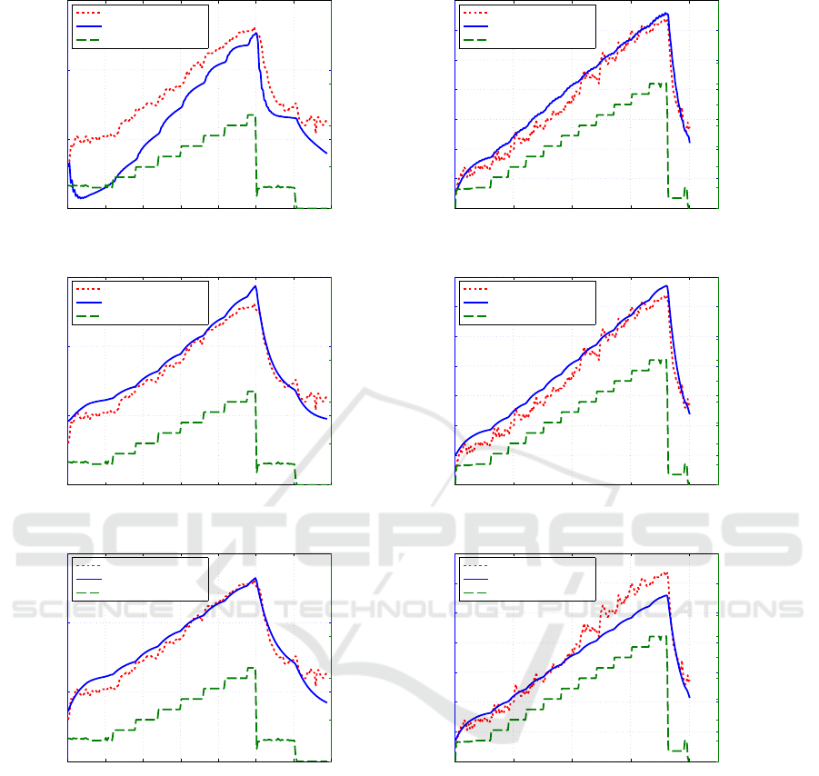
Figure 4: Three typical heart rate prediction examples for label (1) Takagi-Sugeno model, (2) Convolution model, (3) Convo-

lution model with one parameter. Sets a and b illustrated two different experiments, but the same predicted training session

each for all three models.

deal with the same prediction setting, with numbers 7,

9, 10, 22, 23 and 24 leading the way.

As an example, prediction 21 and 22 are visual-

ized in Figure 4, where strain is given in watt and

measured heart rate is plotted against predicted heart

rate for better comparison of model accuracies. Here,

each column shows ﬁgures computed with these three

models but using the same data set. The ﬁgures in

the ﬁrst row are predictions executed from Takagi-

Sugeno, the second row illustrates predictions using

the four parameter Convolution model, and the last

row presents prediction results from the one param-

eter Convolution model approach. While set a illus-

trates an example (no. 22) where the error of Takagi-

Sugeno model is huge, in comparison to Convolution

model approaches, which can both deal with this set-

ting, set b illustrates an example (no. 21) where the

error of all three models is in a similar range, but

the one parameter Convolution model performs a bit

worse than the others.

icSPORTS 2016 - 4th International Congress on Sport Sciences Research and Technology Support

162

4.2 Evaluation and Discussion

Comparison of the Convolution model against known

analytical models has shown that the Convolution

model yields a comparable or even better accuracy.

The Convolution model with one parameter seems to

bring further enhancement. The experiments show

that restrictions to the parameter area can actually im-

prove prediction accuracy. At least, it seems to be rea-

sonable to set the level parameter a

to an individual

resting heart rate value. Since the error in experiment

number 8 is only slightly higher than the error in ex-

periment number 2, the advantages of one parameter

instead of three should be considered: computation is

much faster, ﬁtting is more stable and risks of local

minima are reduced because of the reduced complex-

ity. Since the linkage of a

and a

using a polyno-

mial of the ﬁfth degree yields slightly smaller errors

compared to using the presented polynomial of the

second degree, this linkage combined with the other

two parameter speciﬁcations might be a valid option,

too. But since the average deviation is comparably

small, we decided to uphold the model as simple as

reasonable possible. Therefore we preferred this one

parameter model against the other possibilities.

Given, however, that the training zone for aero-

bic and anaerobic training are approximately 15 to

20 bpm wide (10% of the maximum heart rate), such

a prediction accuracy would not be sufﬁcient. For a

detailed training plan, an accuracy of 5% of the max-

imum heart rate is desired—which can be achieved

using the Convolution model, which yields an error

of around 9 bpm (approach with four parameters) or

7 bpm (approach with one parameter).

In some cases, especially the ﬁrst minutes of train-

ing show huge deviation between the measured and

the predicted heart rate values. By neglecting ﬁrst

minutes of a prediction, the accuracy can be im-

proved. But since this is the case for all models, we ig-

nored this potential improvement and took these ﬁrst

stages into account without exception.

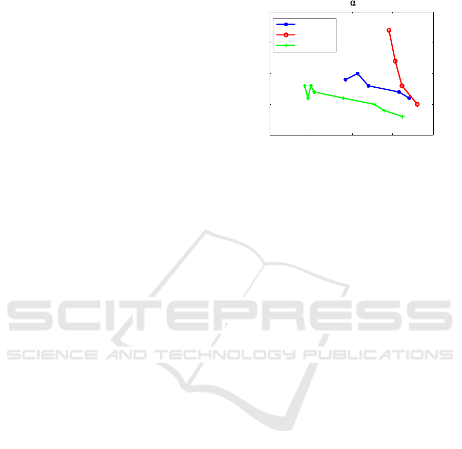
The Convolution model with only one parameter

not only yields good prediction results but also al-

lowed the changes in this remaining parameter for

each subject over time to be observed. In doing so,

the remaining parameter seems to correspond to the

ﬁtness process itself. Figure 5 shows that—apart from

some peaks in the beginning for two subjects—the

value of this parameter decreases while the subject’s

training program continues. Since the subjects re-

ported that they had trained regularly during the ex-

periment period, the measured behavior might explain

their increased ﬁtness. This assumption is based on a

few data only, hence the results will need to be vali-

Jul 2014 Oct 2014 Jan 2015 Apr 2015 Jul 2015

1.5

2.5

3.5

x 10

- 3

subject 1

subject 2

subject 3

Parameter over time

Figure 5: The remaining parameter over time for all three

subjects.

dated using more and larger data sets. At the moment,

the remaining parameter as ﬁtness indicator can only

be taken as a conceptual idea that needs further inves-

tigation.

Regarding other than cycling sports, ﬁrst experi-

ments in running were conducted: Using data of one

male athlete, six exercises performed on a treadmill

were performed. Predicting the heart rate in these

running data results in a median RMSE of 10.68 ±

6.37 bpm using the Takagi-Sugeno model and in a

median RMSE of 6.49 ± 2.35 bpm using the Convo-

lution model with four parameters, indicating that the

Convolution model is applicable to other sports than

cycling as well.

5 CONCLUSION AND FUTURE

WORK

This work presented a new model for heart rate pre-

diction. First of all, a comparison to other heart rate

models was performed. It has been shown that the

Convolution model can fairly compete with other an-

alytical models for predicting the heart rate a whole

training session in advance. Moreover, reducing the

number of arbitrary parameters leads to even smaller

errors and more stability. First experiments on the re-

maining parameter lead us to the assumption that this

parameter might indicate the actual ﬁtness condition

of a subject.

An important next step will be to analyze the use-

fulness of this model in simulating outdoor workouts.

Many cyclists have their well-known training routes

or plan their ride in advance. Therefore, a previous

simulation based on strain according to GPS proﬁles

might be beneﬁcial in training planning.

Additionally, the usefulness of the Convolution

model should be investigated for other sports compre-

A Convolution Model for Heart Rate Prediction in Physical Exercise

163

hensively, such as cycling on other protocols, cycling

without any protocol, running with or without proto-

col, and others.

Furthermore, experiments using a larger data set

with more subjects have to show if a correlation be-

tween changes in ﬁtness and in the remaining Con-

volution model parameter α can be consistently ob-

served.

ACKNOWLEDGEMENT

This work was supported by a funding of the state

North Rhine-Westphalia, Germany.

REFERENCES

Achten, J. and Jeukendrup, A. E. (2003). Heart rate moni-

toring. Sports medicine, 33(7):517–538.

Baig, D.-e.-Z., Su, H., Cheng, T. M., Savkin, A. V., Su,

S. W., and Celler, B. G. (2010). Modeling of human

heart rate response during walking, cycling and row-

ing. In Engineering in Medicine and Biology Soci-

ety (EMBC), 2010 Annual International Conference

of the IEEE, pages 2553–2556. IEEE.

Borresen, J. and Lambert, M. I. (2008). Autonomic con-

trol of heart rate during and after exercise. Sports

medicine, 38(8):633–646.

Brzostowski, K., Drapala, J., and Swiatek, J. (2013). Data-

driven models for ehealth applications. International

Journal of Computer Science and Artiﬁcial Intelli-

gence, 3(1):1–9.

Busso, T., Denis, C., Bonnefoy, R., Geyssant, A., and La-

cour, J.-R. (1997). Modeling of adaptations to phys-

ical training by using a recursive least squares algo-

rithm. Journal of applied physiology, 82(5):1685–

1693.

Calvert, T. W., Banister, E. W., Savage, M. V., and Bach, T.

(1976). A systems model of the effects of training on

physical performance. IEEE Transactions on Systems,

Man and Cybernetics, 6(2):94–102.

Cheng, T. M., Savkin, A. V., Celler, B. G., Wang, L., and

Su, S. W. (2007). A nonlinear dynamic model for

heart rate response to treadmill walking exercise. In

29th Annual International Conference of the IEEE En-

gineering in Medicine and Biology Society (EMBS),

pages 2988–2991. IEEE.

uller, M., Meenakshi Sundaram, A., Ludwig, M., Aster-

oth, A., and Prassler, E. (2015). Modeling and pre-

dicting the human heart rate during running exercise.

In Information and Communication Technologies for

Ageing Well and e-Health, volume 578, pages 106–

125. Springer International Publishing.

Koenig, A., Somaini, L., and Pulfer, M. (2009). Model-

based heart rate prediction during lokomat walking.

Engineering in Medicine and Biology Society, 2009.

EMBC 2009. Annual International Conference of the

IEEE.

Le, A., Jaitner, T., Tobias, F., and Litz, L. (2008). A dy-

namic heart rate prediction model for training opti-

mization in cycling (p83). In The Engineering of Sport

7, pages 425–433. Springer.

Lehmann, M., Foster, C., and Keul, J. (1993). Overtrain-

ing in endurance athletes: a brief review. Medicine &

Science in Sports & Exercise.

Leitner, T., Kirchsteiger, H., Trogmann, H., and del Re, L.

(2014). Model based control of human heart rate on

a bicycle ergometer. In Control Conference (ECC),

2014 European, pages 1516–1521. IEEE.

Ludwig, M., Sundaram, A. M., F

uller, M., Asteroth, A.,

and Prassler, E. (2015). On modeling the cardiovascu-

lar system and predicting the human heart rate under

strain. In Proceedings of the 1st International Confer-

ence on Information and Communication Technolo-

gies for Ageing Well and e-Health (ICT4AgingWell),

pages 106 – 117.

Mohammad, S., Guerra, T. M., Grobois, J. M., and Hec-

quet, B. (2011). Heart rate control during cycling exer-

cise using takagi-sugeno models. In 18th IFAC World

Congress, Milano (Italy), pages 12783–12788.

Paradiso, M., Pietrosanti, S., Scalzi, S., Tomei, P., and Ver-

relli, C. M. (2013). Experimental heart rate regulation

in cycle-ergometer exercises. IEEE Transactions on

Biomedical Engineering, 60(1):135–139.

Refaeilzadeh, P., Tang, L., and Liu, H. (2009). Cross-

validation. In Encyclopedia of database systems,

pages 532–538. Springer.

Smith, L. L. (2003). Overtraining, excessive exercise, and

altered immunity. Sports Medicine, 33(5):347–364.

Su, S. W., Huang, S., Wang, L., Celler, B. G., Savkin, A. V.,

Guo, Y., and Cheng, T. M. (2010). Optimizing heart

rate regulation for safe exercise. Annals of biomedical

engineering, 38(3):758–768.

Su, S. W., Wang, L., Celler, B. G., Savkin, A. V., and Guo,

Y. (2007). Identiﬁcation and control for heart rate reg-

ulation during treadmill exercise. IEEE Transactions

on Biomedical Engineering, 54(7):1238–1246.

Sumida, M., Mizumoto, T., and Yasumoto, K. (2013). Esti-

mating heart rate variation during walking with smart-

phone. In Proceedings of the 2013 ACM international

joint conference on Pervasive and ubiquitous comput-

ing, pages 245–254. ACM.

icSPORTS 2016 - 4th International Congress on Sport Sciences Research and Technology Support

164