
Determining the Near Optimal Architecture of Autoencoder using
Correlation Analysis of the Network Weights
Heng Ma, Yonggang Lu* and Haitao Zhang
School of Information Science and Engineering, Lanzhou University, Gansu, 730000, China
Keywords: Deep Learning, Autoencoder, Architecture Optimization, Correlation Analysis.
Abstract: Currently, deep learning has already been successfully applied in many fields such as image recognition,
recommendation systems and so on. Autoencoder, as an important deep learning model, has attracted a lot
of research interests. The performance of the autoencoder can greatly be affected by its architecture. How-
ever, how to automatically determine the optimal architecture of the autoencoder is still an open question.
Here we propose a novel method for determining the optimal network architecture based on the analysis of
the correlation of the network weights. Experiments show that for different datasets the optimal architecture
of the autoencoder may be different, and the proposed method can be used to obtain near optimal network
architecture separately for different datasets.
1 INTRODUCTION
Since the concept of deep learning was proposed
(Hinton and Salakhutdinov, 2006), it has become
one of the hottest research topics in the machine
learning field. And it has been widely applied in
various fields, such as natural language processing
(NLP) (Collobert and Weston, 2008), image recog-
nition (Ciresan et al., 2012), recommendation sys-
tems (Van den Oord et al., 2013), bioinformatics
(Chicco et al., 2014), and so on. The successful
application of these research projects in the industry
also illustrates the great advantage of deep learning
(Levine et al., 2016).
Deep learning is a method based on several mod-
els of neural networks (autoencoder and MLP).
However, although the performance of deep learning
is greatly dependent on the network architecture, the
current deep learning methods can't adaptively ad-
just the number of layers and the nodes of each lay-
er. In fact, the same problem also exists in the early
age of the research on neural network, so many
sophisticated methods have been put forward to
optimize architecture of neural network (Reiter-
manova, 2008).
The most common approach is brute-force meth-
od (Reed, 1993). This method tries all kinds of net-
work architecture in a reasonable range, and finally
*Corresponding author
finds an optimal architecture that is suitable for
training datasets. Because of the high computational
complexity, people seldom use this method directly.
The pruning algorithms (Reed, 1993) is another
method, its principle is to remove the redundant
parts of network through certain indicators. The
concrete implementation of pruning method is as
follows: weight saliency (Mozer et al.. 1989), opti-
mal brain damage (OBD) (LeCun et al., 1989), op-
timal brain surgeon (OBS) (Hassibi et al., 1993), etc.
The only difference among these methods is to use
different strategies for computing indicators. Since
indicator calculation is based on error function, the
main drawback of pruning methods is high computa-
tional complexity. Network construction technique
(Lee, 2012) can also be used to optimize architec-
ture. It begins with a minimal network, then dynam-
ically adds and trains hidden units until a satisfacto-
ry architecture is reached. The cascade correlation
method (Fahlman and Lebiere, 1989) is a famous
representative of this technique. This method has the
following advantages: training is fast, being useful
for incremental learning, results can be cached, and
so on. But the disadvantages are also obvious: its
candidate nodes are independent, and the interac-
tions between related nodes are not considered. So it
is only suitable for networks with relatively simple
architecture. There are many other techniques, for
example, probability optimization techniques and
regularization techniques (Reitermanova, 2008).
Ma, H., Lu, Y. and Zhang, H.
Determining the Near Optimal Architecture of Autoencoder using Correlation Analysis of the Network Weights.
DOI: 10.5220/0006039000530061
In Proceedings of the 8th International Joint Conference on Computational Intelligence (IJCCI 2016) - Volume 3: NCTA, pages 53-61
ISBN: 978-989-758-201-1
Copyright
c
2016 by SCITEPRESS – Science and Technology Publications, Lda. All rights reserved
53

However, these methods are also only suitable for
optimizing simple network, for example, the net-
work with one hidden layer and small number of
nodes. Recently, genetic algorithms are widely used
to optimize network architecture and weights (Fisze-
lew et al., 2007). But its slow convergence rate is a
very influential factor. So corresponding to complex
deep learning models with many hidden layers, new
methods need to be developed for the architecture
optimization.
The proposed architecture optimization method
in the paper is specifically aimed at the complex
deep learning model with many hidden layers and a
large number of nodes, which can adjust the number
of the nodes in multiple hidden layers. To improve
the efficiency, the optimization is based on the cor-
relation analysis of the node weights initialized us-
ing the Restricted Boltzmann Machine (RBM) (Hin-
ton and Salakhutdinov, 2006). Different from the
traditional methods, the time-consuming network
training process is avoided in the proposed architec-
ture optimization method.
The proposed method has the following ad-
vantages: First, it can be well applied to the complex
network architecture optimization. Because the
computing unit of the method is the set of multiple
nodes rather than a single node, the method can be
easily extended for the network with a lot of layers.
Second, the proposed architecture optimization is
based on the correlation analysis between the
weights of the nodes after initialization rather than
the error function after training, the efficiency is
greatly improved.
The rest of paper is organized as follows. In Sec-
tion 2, we first briefly introduce the working flow of
deep learning model and the mechanism of RBM in
network initialization. And then we discuss in detail
about the calculation of correlation coefficient in
Subsection 2.1. At last, Subsection 2.2 shows the
detailed steps of method about optimizing multiple
hidden layer nodes. In Section 3, we present the
experimental results through analyzing and compar-
ing different datasets. Finally, Section 4 draws con-
clusions and discusses the future research direction.
2 ARCHITECTURE
OPTIMIZATION METHOD
Autoencoder, as a kind of deep learning model, is
often used for dimensionality reduction (Laurens
van der Maaten et al., 2009). Our proposed method
is based on this model framework. It consists of the
encoder module which transforms high dimensional
input data into low dimensional output data (code),
and the decoder module which reconstructs the high
dimensional data from the code. The construction of
the autoencoder is mainly concentrated on the en-
coder module because the decoder module can be
approximately regarded as transposition of the en-
coder module. Our method is to optimize the struc-
ture of the encoder module. In the training of deep
learning, RBM is used to initialize the weights of the
nodes. The usage of RBM is a significant improve-
ment of the deep learning model because it is diffi-
cult to optimize the weights of the nodes of the mul-
tiple hidden layers without good initial weights
(Hinton and Salakhutdinov, 2006).
RBM is a kind of stochastic two-layer network
containing a visible layer corresponding to the input
and a hidden layer corresponding to the output. The
two layers are fully connected, that is to say, each
node of the hidden layer connects to all the nodes of
the visible layer, but the nodes in the same layer
cannot connect to each other. In the initialization
process, the network will be divided into multiple
RBMs and the output of previous RBM will become
the input of the next RBM, so as to achieve the ex-
traction of input data information layer by layer.
The second step is the weights fine-tuning after
RBM initialization. Using the traditional weights
fine-tuning methods, for example, backpropagation
(BP), can fine-tune weights by minimizing the data
reconstruction error.
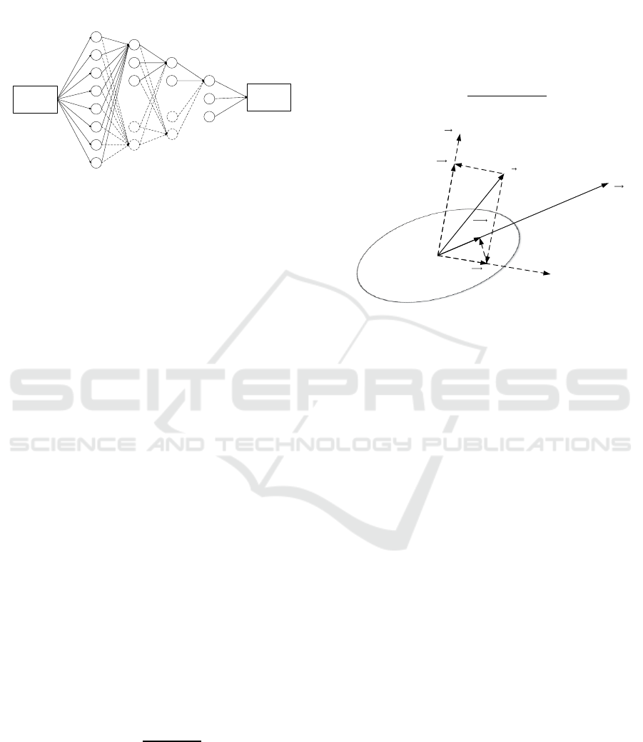
The proposed network architecture optimization
method working on the above framework is depicted
in Figure 1. In the initial stage, a simple network
with very small number of nodes in each hidden
layer is created, which corresponds to the architec-
ture of nodes connected by solid lines in Figure 1.
The architecture optimization is achieved by dynam-
ic growth of the number of the nodes of the hidden
layers, where the added nodes correspond to the
nodes connected by dotted lines in Figure 1. At each
step, the same number of nodes (N
i
nodes) are added
to the target layer, then the correlation analysis on
the weights of all the nodes (the weights of the node
stand for the weights between all the nodes of the
previous layer and the current node) in the layer is
carried out. In our method, N
i
nodes which have the
smallest correlation with the rest of the nodes are
selected from all the nodes. The correlation coeffi-
cient between the selected nodes and the rest of the
nodes are computed (See Subsection 2.1 for details).
At the end, when the correlation coefficient is great-
er than a given threshold, the dynamic growth of the
number of the nodes is stopped and the number of
NCTA 2016 - 8th International Conference on Neural Computation Theory and Applications
54
the nodes for the layer is determined. For the next
hidden layer, the above process is repeated. Detailed
implementation is introduced in Subsection 2.2.
Figure 1: Illustration of the architecture optimization. The
nodes connected by solid lines are the original nodes. The
nodes connected by the dotted lines are the added nodes.
2.1 Correlation Coefficient between
Two Sets of the Nodes
The definition of correlation coefficient between two
sets of nodes is the theoretical basis of our method.
The correlation coefficient is used to analyze the
relationship between one group of nodes called
Main_Nodes and the other group of nodes called
Other_Nodes in the same layer. In the first step, we
get S nonzero eigenvalues called SltedValues and
the corresponding eigenvectors called SltedVectors
of the weights of the Main_Nodes by principal com-
ponent analysis (PCA), and then construct the prin-
cipal component space (PCS) using the SltedVectors
(Figure 2). The unit vectors of the SltedVectors are
represented as
, while the correspond-
ing eigenvalues called SltedValues are represented
as {
1
,
2
, …,
S
}. If the weights of Other_Nodes
are represented as
, the projection of
to the prin-
cipal component space, represented as
, can be
derived from:
(1)
The vertical component
is defined as:
(2)
Given
and
, we can calculate the main correla-
tion coefficient by the following formula:
(3)
The above formula only concerns with the direction
relations between
and PCS, while the SltedValues
computed from Main_Nodes are ignored. So another
correlation coefficient is defined in formula (4)
which gives main components more weights. For the
correlation between
and
which is the dominant
component, the largest eigenvalue is used as the
weight. If the directions of
and
is more con-
sistent (the greater value of
), the correlation
coefficient is greater.
(4)
Figure 2: Illustration of correlation coefficient. The princi-
pal component space (PCS) is constructed from SltedVec-
tors.
is the vertical direction to the principal component
space.
is the dominant component.
is the weights of the
Other_Nodes.
and
are the projections of
on
and
PCS respectively.
is the projection of
to
.
The overall correlation coefficient is given by the
following formula:
(5)
where stands for the ratio parameter. In order to
determine the value of , we conduct experiments
by changing the value of from 0 to 1. It is found
that is a good choice.
The pseudo code for calculating the correlation
coefficient between two given node sets is shown in
Figure 3.
2.2 Architecture Optimization
In this subsection, how the correlation coefficient is
used to realize architecture optimization is de-
scribed. The process of architecture optimization is
divided into two steps, the first step is to compute
the correlation coefficient, and the second step is to
control the growth of the nodes by comparing the
correlation coefficient with a given threshold.
In the first step, RBM initialization on the cur-
rent hidden layer containing both the added nodes
and the original nodes will be carried out in order to
obtain the weights of the nodes. Then the correlation
Decoder
module
Input
data
...
...
Hidden
layer 1
Hidden
layer 2
Hidden
layer 3
Output
layer
V
D
I
Principal
Component
Space
V
I
P
I
PD
I
Determining the Near Optimal Architecture of Autoencoder using Correlation Analysis of the Network Weights
55

Figure 3: The pseudo code of calculating correlation coefficient.
coefficient of the weights of the layer is computed as
introduced in Subsection 2.1.
In the second step, the architecture optimization
on the autoencoder model is carried out. The pseudo
code for the architecture optimization is shown in
Figure 4.
3 EXPERIMENTS
The method is implemented using Matlab. In order
to verify the performance of the proposed method,
the following datasets are used: MNIST, USPS,
Binary Alphadigits and MFEAT. The first three
datasets are available at: http://www.cs.nyu.edu/
~roweis/data.html. The MFEAT dataset is available
at: http://archive.ics.uci.edu/ml/datasets.html.
The MNIST dataset is a dataset of handwritten
digits (0-9), it contains 70000 images of size 2828.
Considering the high computational cost, 250 sam-
ples of each class are selected as the training set, and
50 samples of each class are selected as the test set.
The USPS dataset is another handwritten digits
dataset which contains images of size 1616 and
there are 1100 samples in each class. As same as
MNIST, 250 samples of each class are selected as
the training set, and other 50 samples of each class
are selected as the test set.
The Binary Alphadigits dataset is a handwritten
alphabet and digits dataset. It contains a total of 36
classes from “1” to “9”, and “A” to “Z", the size of
the image is 2016 and each class contains 39 sam-
ples. For 39 images of each class, 33 images are
used as the training set and 6 images as the test set.
The MFEAT dataset is also a handwritten nu-
merals dataset which contains ten classes from "0" to
"9". The size of image is 1615 and each class con-
tains 200 samples. For 200 images of each class, 150
images are used as the training set and 50 other
images as the test set.
CalculateCorr(Main_Nodes, Other_Nodes, ) {
// Input: Main_Nodes: the input set of the nodes used to construct the
// Other_Nodes: the input set of the Nodes projected to the
// : the ratio parameter
// Output: the correlation coefficient between Main_Nodes and Other_Nodes
// Notes: the weights attribute of a node stands for the weights between the node and all
// the nodes of the previous layer, M stands for the number of the nodes of the
// previous layer.
Main_NodeWeights[1...N1, 1...M] Main_Nodes.weights;
Other_NodeWeights[1...N2,1...M] Other_Nodes.weights;
[Eigenvectors[1...M,1...M], Eigenvalues[1...M]] PCA(Main_NodeWeights);
[SltedVectors[1...M,1...S], SltedValues[1...S]] remove zero eigenvalues and the
corresponding eigenvectors from [Eigenvectors, Eigenvalues];
for i 1 to N2 do {
PerRow_Other_Normalized normalize each row of Other_NodeWeights;
for j 1 to S do {
Parallel_Main(j,:) ;
Parallel_Tune(j) ;
}
Parallel the sum of the Parallel_Main by rows;
Vertical Other_NodeWeights(i,:) - Parallel;
corr_main ;
corr_tune ;
Result(i) ;
}
retur n the mean of Result;
}
PCS
PCS
2
_ (:, )
(:, )
(:, )
T
Other NodeWeights SltedVectors j
SltedVectors j
SltedVectors j
Parallel
Parallel Vectical
_.Parallel Tune SltedValues
SltedValues
_ ( (1 ) _ )corr main corr tune
_ _ (:, )
(:, )
PerRow Other Normalized SltedVectors j
SltedVectors j
NCTA 2016 - 8th International Conference on Neural Computation Theory and Applications
56

Figure 4: The pseudo code of architecture optimization.
The initial network architecture is set to 1000-
200-50-30 in all the experiments. The size of the 1st
hidden layer is fixed at 1000, and the number of the
nodes in the 2nd and the 3rd hidden layers are in-
creased from the initial sizes which are 200 and 50
respectively to determine the near optimal number of
the nodes in the experiments.
3.1 Parameter Selection
In this subsection, the effects of different RBM
training epochs on our method are compared using
multiple datasets, and a good threshold of the corre-
lation coefficient is derived. The final autoencoder
architecture generated through our method is com-
pared with the standard architecture (1000-500-250-
30) used in (Hinton and Salakhutdinov, 2006). The
parameters of RBM are listed below: learning rate
for weights
=0.1, learning rate for biases of visi-
ble units
=0.1, learning rate for biases of hidden
units
=0.1, the weight cost is 0.0002, the initial
momentum is 0.5, the final momentum is 0.9, and
learning is done with 1-step Contrastive Divergence.
At the same time, we adjust the training epoch of
backpropagation from 200 to 20, because it is found
that in the standard autoencoder framework, the
reconstruction error becomes steady when the train-
ing epoch reaches above 15.
In order to analyze the relationship between the
correlation coefficients and the number of nodes, we
first fix nodes number of the 2nd hidden layer to
500, then increase the number of the nodes of the
3nd hidden layer from 50 to 500, and the number of
nodes added at each step is 25. We also set 5 differ-
ent RBM training epochs, 10, 50, 100, 300 and 500,
respectively. The results are shown in Figure 5.
As can be seen from Figure 5, under the different
RBM training epochs, the correlation coefficient
curve has a similar trend, in the initial stage of in-
creasing the number of nodes, the correlation coeffi-
ArchitectureOptimization(Nodes2, n2, Nodes3, n3, max_n2, nInc, TH) {
// Nodes2: the nodes of the 2nd hidden layer
// n2: the initial number of the nodes of the 2nd hidden layer
// Nodes3: the nodes of the 3rd hidden layer
// n3: the initial number of the nodes of the 3rd hidden layer
// max_n2: the max number of the nodes of the 2nd hidden layer
// nInc: the increment of the number of the nodes at each step
// TH: the threshold of the correlation coefficient
Nodes2.Num_Nodes n2;
Nodes3.Num_Nodes n3;
OptimizeLayer(Nodes2, max_n2, nInc, TH);
// max_n3 is the max number of the nodes of the 3rd hidden layer;
max_n3 Nodes2.Num_Nodes;
OptimizeLayer(Nodes3, max_n3, nInc, TH);
}
OptimizeLayer(Nodes, max_num_nodes, nInc, TH) {
while Nodes.Num_Nodes < max_num_nodes do {
Nodes.Num_Nodes Nodes.Num_Nodes + nInc;
initialize the weights of the Nodes using RBM;
for i 1 to Nodes.Num_Nodes do {
// calculating the correlation coefficient between
// each node and the remaining nodes
Corr_Each[i] CalculateCorr(Nodes-{Nodes[i]}, {Nodes[i]}, 0.8) ;
}
SltedNodes the nInc nodes having the largest Corr_Each values;
RemNodes Nodes - SltedNodes;
corr CalculateCorr(RemNodes, SltedNodes, 0.8);
if corr > TH then {
Nodes Nodes - SltedNodes;
break;
}
}
}
Determining the Near Optimal Architecture of Autoencoder using Correlation Analysis of the Network Weights
57
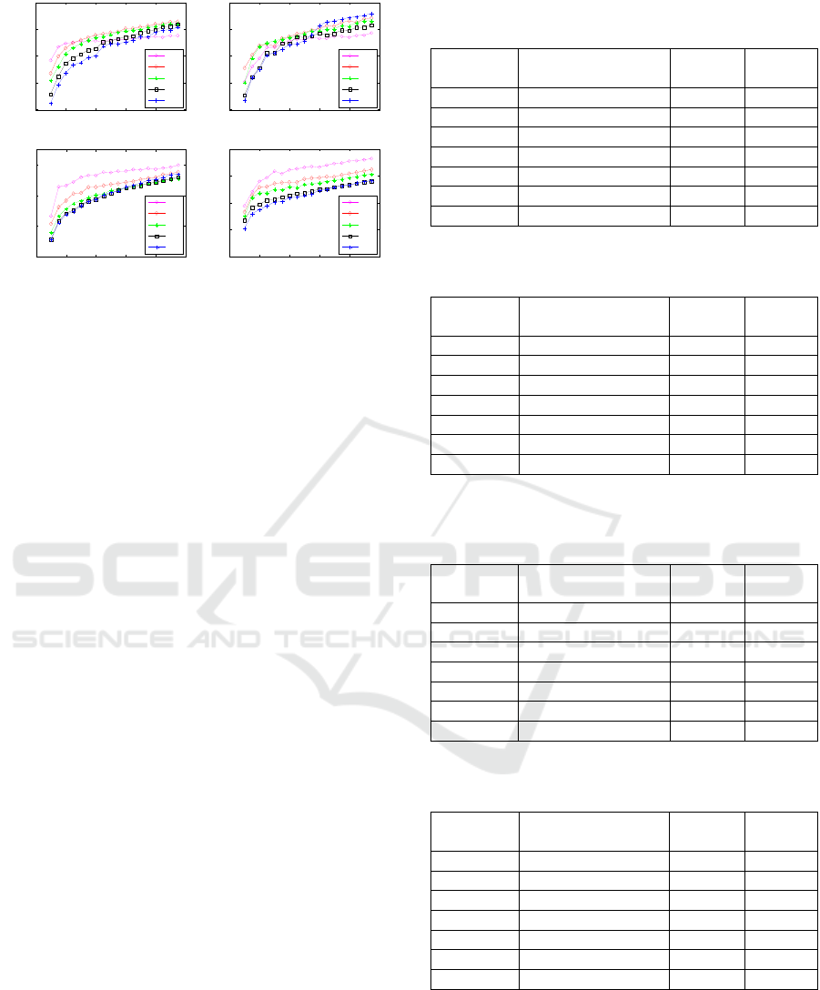
Figure 5: The correlation coefficient curves of MNIST,
USPS, Binary Alphadigits and MFEAT datasets, under
different RBM training epochs.
cient increases rapidly with a large slope value.
When the number of nodes reaches about 250, the
slope of the curve becomes small, and the correlation
coefficient curve is close to steady. In order to bal-
ance computational complexity and reliability of the
results, the value of RBM training epochs is set to
300. The following experiments are all based on this
epoch value. From Figure 5, it is also found that the
threshold of the correlation coefficient will have a
great impact on the final network architecture. So
Table 1, Table 2, Table 3 and Table 4 are used to
show the derived network architecture under differ-
ent thresholds. In tables, "Threshold" stands for the
threshold of correlation coefficient; "Network archi-
tecture", "Training error" and "Test error" are the
experiment results of our method. The last row of
every table is the standard autoencoder architecture.
From Table 1 to Table 4, we can find that differ-
ent correlation coefficient thresholds correspond to
different derived network architecture. With the
increasing of the correlation coefficient threshold,
the number of the nodes of the 2nd and the 3rd layer
increases, and the training error and the test error
both decrease. It can be seen from the tables that a
value of 0.65 for the correlation coefficient divides
the thresholds corresponding to high and low error
values. So it is reasonable to select 0.65 as an appro-
priate value for the threshold of the correlation coef-
ficient.
Based on the analysis of the experiment results,
the RBM training epoch is set to 300 and the thresh-
old of correlation coefficient is set to 0.65. From
Table 1 to Table 4, it is also found that the training
error and the test error have the similar trend with
the increasing of the correlation coefficient threshold,
so only the test errors are used to evaluate the exper-
iments results in Subsection 3.2.1.
Table 1: The derived network architecture under different
thresholds of correlation coefficient for MNIST dataset.
Threshold
Network architecture
Training
error
Test
error
0.75
1000-975-950-30
3.1427
10.8150
0.7
1000-850-425-30
3.3946
11.1748
0.65
1000-650-375-30
3.4251
11.1861
0.6
1000-425-225-30
4.0720
12.0827
0.55
1000-250-100-30
6.2062
14.1175
0.5
1000-200-50-30
10.3525
17.6577
Standard
1000-500-250-30
3.8137
11.6349
Table 2: The derived network architecture under different
thresholds of correlation coefficient for USPS dataset.
Threshold
Network architecture
Training
error
Test
error
0.75
1000-975-950-30
2.0769
4.9900
0.7
1000-825-300-30
2.1622
5.0034
0.65
1000-650-175-30
2.4675
5.2466
0.6
1000-425-75-30
3.4843
6.3163
0.55
1000-200-50-30
5.0167
7.8166
0.5
1000-200-50-30
4.9150
7.6937
Standard
1000-500-250-30
2.2517
4.9890
Table 3: The derived network architecture under different
thresholds of correlation coefficient for Binary Alphadigits
dataset.
Threshold
Network architecture
Training
error
Test
error
0.75
1000-1000-950-30
1.0767
28.6581
0.7
1000-925-725-30
1.4014
28.5264
0.65
1000-825-450-30
1.7354
29.6531
0.6
1000-675-325-30
2.5168
30.4159
0.55
1000-425-225-30
3.8307
31.8818
0.5
1000-250-200-30
5.1563
32.8270
Standard
1000-500-250-30
3.4705
31.0856
Table 4: The derived network architecture under different
thresholds of correlation coefficient for MFEAT dataset.
Threshold
Network architecture
Training
error
Test
error
0.75
1000-1000-950-30
1.4950
6.7036
0.7
1000-900-600-30
1.5700
6.7838
0.65
1000-750-300-30
1.7540
6.8433
0.6
1000-575-225-30
1.9229
7.0369
0.55
1000-325-100-30
2.9155
7.9328
0.5
1000-200-50-30
5.6372
9.7033
Standard
1000-500-250-30
1.9039
6.9822
3.2 Experiment Results and Analysis
By using the parameter values obtained in the last
section, we can get the near optimal network archi-
tecture of four datasets from Table 1 to Table 4. For
MNIST, the selected network structure is 1000-650-
0 100 200 300 400 500
0.3
0.4
0.5
0.6
Node Number (MNIST)
Correlation Coefficient
10
50
100
300
500
0 100 200 300 400 500
0.3
0.4
0.5
0.6
Node Number (USPS)
Correlation Coefficient
10
50
100
300
500
0 100 200 300 400 500
0.3
0.4
0.5
0.6
Node Number (Binary Alphadigits)
Correlation Coefficient
10
50
100
300
500
0 100 200 300 400 500
0.3
0.4
0.5
0.6
Node Number (MFEAT)
Correlation Coefficient
10
50
100
300
500
NCTA 2016 - 8th International Conference on Neural Computation Theory and Applications
58
375-30; for USPS, it is 1000-650-175-30; for Binary
Alphadigits, it is 1000-825-450-30, and for MFEAT,
it is 1000-750-300-30. In order to verify our method
and evaluate these results, reconstruction error and
the correlation coefficient between the distance
matrices of high dimensional raw data and the low
dimensional data (code) are used.
3.2.1 Evaluation using Reconstruction Error
Reconstruction error is a primary evaluation index of
the autoencoder performance. It is calculated by first
decoding these low dimensional codes to obtain the
reconstructed high dimensional data, followed by
computing the error between the reconstructed data
and the original data. We calculated the test error
from the test data using mean square errors (MSE).
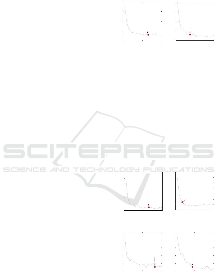
Because the proposed method is used to adjust
both the number of the nodes in the 2nd and the 3rd
hidden layers, we firstly fix the number of the nodes
of the 2nd or the 3rd layer, and then change the
number of the nodes of the other layer. Taking the
test error curves of MNIST dataset shown in Figure
6 as an example, the curve in the left graph is pro-
duced under the condition that the number of the
nodes of the 3rd hidden layer is fixed to 375 and the
number of the nodes of the 2nd hidden layer increas-
es from 50 to 1000 with step 50. The curve in the
right graph is produced under the condition that the
number of the nodes of the 2nd hidden layer is fixed
to 650 and the number of the nodes of the 3rd hid-
den layer increases from 50 to 1000 by 50. In the
Figure 6, the red dot represents the selected optimal
number of the nodes of the current layer. It is found
that the test error curves of the 2nd and the 3rd layer
are both a relatively smooth curve that shows a
downward trend. With the increasing of the number
of the nodes, the slope becomes smaller. The select-
ed optimal number of nodes is located in the rela-
tively flat area of the curves, which indicates that the
method finds a near optimal network architecture for
the MNIST dataset.
The test error curves of USPS dataset are shown
in Figure 7, the test error curves of Binary Alphadig-
its dataset are shown in Figure 8, and the test error
curves of MFEAT dataset are shown in Figure 9. It
is found that the trend of those curves and the loca-
tion of the selected optimal node number are both
very similar to these of the MNIST dataset. So, the
proposed method can also find the near optimal
network architecture for the USPS, Binary Alpha
and MFEAT datasets.
Figure 6: The test error curves of MNIST dataset.
3.2.2 Evaluation using Correlation
Coefficient between Distance Matrices
In this subsection, the correlation coefficient be-
tween the distance matrices of high dimensional
input data and low dimensional code is used to eval-
uate the proposed method. The distance matrix of
high dimensional input data indicates the distribu-
tion relationship between the input samples. And the
distance matrix of low dimensional code indicates
the distribution relationship between the samples
after the dimension reduction. It is obvious that we
can evaluate the network architecture by comparing
the correlation between the two distance matrices.
After the distance matrices are computed using the
Euclidean distance, the Pearson's correlation coeffi-
cient (Stigler, 1989) between them is computed.
High value of the correlation coefficient infers ap-
propriate network architecture.
Figure 7: The test error curves of USPS dataset.
Figure 8: The test error curves of Binary Alphadigits
dataset.
0 500 1000
10
12
14
16
18
Selected Node
Number
Node Number (2nd layer)
Test Error
0 500 1000
10
12
14
16
18
Selected Node
Number
Node Number (3rd layer)
Test Error
0 500 1000
5
5.5
6
6.5
7
7.5
8
Selected Node
Number
Node Number (2nd layer)
Test Error
0 500 1000
4.5
5
5.5
6
6.5
7
7.5
8
Selected Node
Number
Node Number (3rd layer)
Test Error
0 500 1000
28
30
32
34
36
38
Selected Node
Number
Node Number (2nd layer)
Test Error
0 500 1000
28
30
32
34
36
38
Selected Node
Number
Node Number (3rd layer)
Test Error
Determining the Near Optimal Architecture of Autoencoder using Correlation Analysis of the Network Weights
59
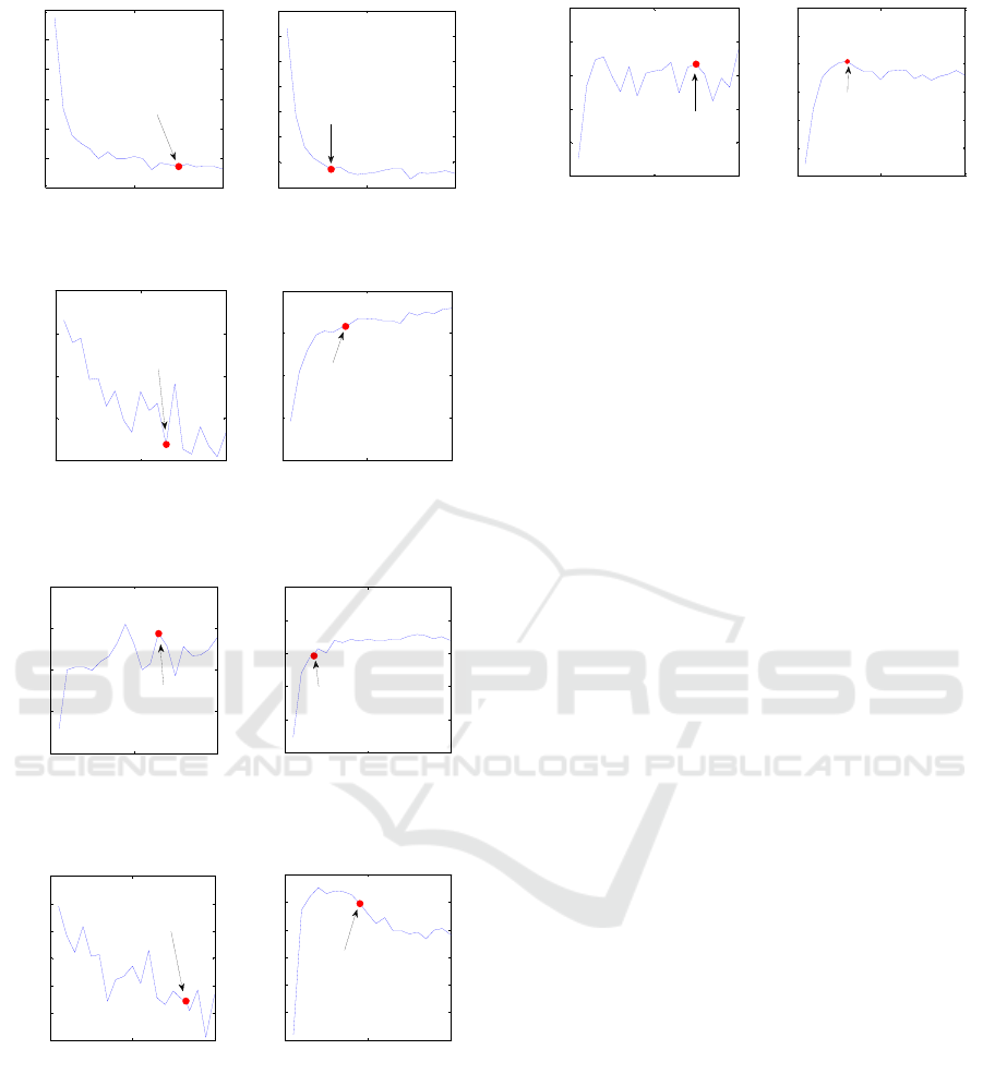
Figure 9: The test error curves of MFEAT dataset.
Figure 10: The correlation coefficient curves of the dis-
tance matrices of MNIST dataset.
Figure 11: The correlation coefficient curves of the dis-
tance matrices of USPS dataset.
Figure 12: The correlation coefficient curves of the dis-
tance matrices of Binary Alphadigits dataset.
The correlation coefficient curves of the distance
matrices of MNIST, USPS, Binary Alphadigits and
MFEAT datasets are shown in Figure 10, Figure 11,
Figure 12 and Figure 13 respectively. From the
figures, it can be seen that for all the four datasets
the curves of the 3rd layer on the right side have the
similar trend: in the early stage of the increasing of
the node number, the correlation coefficient
Figure 13: The correlation coefficient curves of the dis-
tance matrices of MFEAT dataset.
increases rapidly and the slope of the curves is high,
and after the above stage, the curves show a slow
rise or a downward trend, and the selected optimal
nodes number is located in the relatively flat area of
the curves. It is also found that there is no obvious
common trend of the correlation curves of the 2nd
hidden layer for these four datasets. The correlation
coefficient of the 2nd layer is not directly related
with the output of the network. This may be why
there is no common pattern in the correlation curves
of the 2nd layer.
4 CONCLUSIONS
In this paper, we propose an architecture optimiza-
tion method for autoencoder. The method can adap-
tively adjust the number of the nodes of the hidden
layers to find a near optimal architecture of the net-
work for different datasets. The method is based on
the correlation analysis of the network weights after
RBM initialization. The experimental results show
that the proposed method can automatically produce
the near optimal architecture for the autoencoder. In
future work, we plan to analyze the relationship
between the size of the input data and the number of
the nodes in the 1st hidden layer, so that the archi-
tecture optimization of the whole network can be
realized.
ACKNOWLEDGEMENTS
This work is supported by the National Natural Sci-
ence Foundation of China (Grants No. 61272213)
and the Fundamental Research Funds for the Central
Universities (Grants No. lzujbky-2016-k07).
0 500 1000
6.5
7
7.5
8
8.5
9
9.5
Selected Node
Number
Node Number (2nd layer)
Test Error
0 500 1000
6.5
7
7.5
8
8.5
9
9.5
10
Selected Node
Number
Node Number (3rd layer)
Test Error
0 500 1000
0.7
0.72
0.74
0.76
0.78
Selected Node
Number
Node Number (2nd layer)
Correlation Coefficient
0 500 1000
0.4
0.5
0.6
0.7
0.8
Selected Node
Number
Node Number (3rd layer)
Correlation Coefficient
0 500 1000
0.8
0.82
0.84
0.86
0.88
Selected Node
Number
Node Number (2nd layer)
Correlation Coefficient
0 500 1000
0.7
0.75
0.8
0.85
0.9
0.95
Selected Node
Number
Node Number (3rd layer)
Correlation Coefficient
0 500 1000
0.8
0.81
0.82
0.83
0.84
0.85
0.86
Selected Node
Number
Node Number (2nd layer)
Correlation Coefficient
0 500 1000
0.72
0.74
0.76
0.78
0.8
0.82
0.84
Selected Node
Number
Node Number (3rd layer)
Correlation Coefficient
0 500 1000
0.935
0.94
0.945
0.95
0.955
0.96
Selected Node
Number
Node Number (2nd layer)
Correlation Coefficient
0 500 1000
0.91
0.92
0.93
0.94
0.95
0.96
0.97
Selected Node
Number
Node Number (3rd layer)
Correlation Coefficient
NCTA 2016 - 8th International Conference on Neural Computation Theory and Applications
60

REFERENCES
Chicco, D., Sadowski, P., & Baldi, P. 2014. Deep autoen-
coder neural networks for gene ontology annotation
predictions. In Proceedings of the 5th ACM Confer-
ence on Bioinformatics, Computational Biology, and
Health Informatics. ACM. pp. 533-540.
Ciresan, D., Meier, U., & Schmidhuber, J. 2012. Multi-
column deep neural networks for image classification.
In Computer Vision and Pattern Recognition (CVPR),
2012 IEEE Conference. IEEE. pp. 3642-3649.
Collobert, R., & Weston, J. 2008. A unified architecture
for natural language processing: Deep neural networks
with multitask learning. In Proceedings of the 25th in-
ternational conference on Machine learning. ACM.
pp. 160-167.
Fahlman, S. E. and Lebiere, C., 1990, The cascade-
correlation learning architecture, in Advances in NIPS,
edited by D. S. Touretzky, vol. 2, pp. 524–532.
Fiszelew, A., Britos, P., Ochoa, A., Merlino, H., Fernán-
dez, E., & García-Martínez, R. 2007. Finding optimal
neural network architecture using genetic algorithms.
Advances in computer science and engineering re-
search in computing science, 27, pp. 15-24.
Hassibi, B., Stork, D. G., & Wolff, G. J. 1993. Optimal
brain surgeon and general network pruning. In Neural
Networks, 1993., IEEE International Conference.
IEEE. pp. 293-299.
Hinton, G. E., & Salakhutdinov, R. R. 2006. Reducing the
dimensionality of data with neural networks. Science,
313(5786), pp. 504-507.
Laurens van der Maaten, Eric Postma & Jaap van den
Herik. 2009. Dimensionality reduction: A comparative
review. Tilburg, Netherlands: Tilburg Centre for Crea-
tive Computing, Tilburg University, Technical Report:
2009-005.
LeCun, Y., Denker, J. S., Solla, S. A., Howard, R. E., &
Jackel, L. D. 1989. Optimal brain damage. In Advanc-
es in NIPS, vol. 2, pp. 598-605.
Lee, T. C. 2012. Structure level adaptation for artificial
neural networks (Vol. 133). Springer Science & Busi-
ness Media.
Levine, S., Pastor, P., Krizhevsky, A., & Quillen, D. 2016.
Learning Hand-Eye Coordination for Robotic Grasp-
ing with Deep Learning and Large-Scale Data Collec-
tion. arXiv preprint arXiv:1603.02199.
Mozer, M. C., & Smolensky, P.. Skeletonization. 1989. A
technique for trimming the fat from a network via rel-
evance assessment. In Advances in Neural Information
Processing Systems. pp. 107-115.
Reed, R. 1993. Pruning algorithms-a survey. IEEE Trans-
actions on Neural Networks, 4(5), pp. 740-747.
Reitermanova, Z. 2008. Feedforward neural networks–
architecture optimization and knowledge extraction.
WDS’08 proceedings of contributed papers, Part I, pp.
159-164.
Stigler, S. M. 1989. Francis Galton's account of the inven-
tion of correlation.Statistical Science, pp. 73-79.
Van den Oord, A., Dieleman, S., & Schrauwen, B. 2013.
Deep content-based music recommendation. In Ad-
vances in Neural Information Processing Systems. pp.
2643-2651.
Determining the Near Optimal Architecture of Autoencoder using Correlation Analysis of the Network Weights
61
