
Training Simulation with Nothing but Training Data
Simulating Performance based on Training Data
Without the Help of Performance Diagnostics in a Laboratory
Melanie Ludwig, David Schaefer and Alexander Asteroth
Computer Science Department, Bonn-Rhein-Sieg University o.A.S., Grantham-Allee 20, 53757 St. Augustin, Germany
Keywords:
Training Model, Performance Simulation, Model Fitting, Field Study.
Abstract:
Analyzing training performance in sport is usually based on standardized test protocols and needs laboratory
equipment, e.g., for measuring blood lactate concentration or other physiological body parameters. Avoiding
special equipment and standardized test protocols, we show that it is possible to reach a quality of performance
simulation comparable to the results of laboratory studies using training models with nothing but training data.
For this purpose, we introduce a fitting concept for a performance model that takes the peculiarities of using
training data for the task of performance diagnostics into account. With a specific way of data preprocessing,
accuracy of laboratory studies can be achieved for about 50% of the tested subjects, while lower correlation of
the other 50% can be explained.
1 INTRODUCTION
It is widely accepted that the right dose of exercise is
a very important factor in efficient training. However,
the right dose strongly depends on each individual and
may change during training periods. Professional ath-
letes therefore have a coach, trainer, sport scientist, or
are under doctoral maintenance and their exercise ses-
sions are individually supervised and controlled by a
professional.
Professional coaches make use of the athlete’s
physiological data, e.g., blood lactate concentration
or
˙
VO
2
max, measured during standardized test pro-
tocols. Based on this data the current athlete’s per-
formance level is assessed and an appropriate training
plan is generated. To put it the other way round, an ap-
propriate training plan is mostly dependent on partic-
ular equipment and a specialist interpreting measured
data and generating a plan.
But not only athletes and professionals are inter-
ested in appropriate and individual training plans. For
amateur athletes and in leisure sports, the usage of
activity tracking systems is increasing these days as
cited in (Krebs and Duncan, 2015). With these appli-
cations they can track their activities and analyze past
training sessions—with more or less accuracy (Yang
et al., 2015; Lee et al., 2014). But so far they can not
accurately predict the progress of training nor create
a suitable training plan including next steps to do.
Regarding outdoor cycling performance, (Balmer
et al., 2000) found peak power for a certain time to be
a useful predictor. Furthermore, (Tan and Aziz, 2005)
found that laboratory determined absolute peak power
might predict cycling performance on a flat course,
and that relative peak power seems to be a useful pre-
dictor of performance during uphill cycling. But here,
too, laboratory tests are necessary beforehand in order
to predict the outdoor cycling performance.
Therefore, the goal of this study was to exam-
ine the feasibility in simulating performance—which
can be used for generating individual training plans—
without invasive methods like blood lactate measur-
ing, coaches, laboratory studies, or any other special
equipment. As a first step towards this direction and
to compare the results to the results of laboratory stud-
ies, the method was tested on ambitious (leisure) cy-
clists only.
Recently, (Schaefer et al., 2015) described a
method for generating individual training plans based
on the Fitness-Fatigue model (Calvert et al., 1976),
a common antagonistic model for performance diag-
nostics.
Using the traipor concept, this paper presents
a new possibility in preprocessing non-standardized
data before fitting necessary model parameters to an
individual without any laboratory measurements or
invasive methods. Combined with generating training
plans, ambitious sportsperson can easily figure out an
Ludwig, M., Schaefer, D. and Asteroth, A.
Training Simulation with Nothing but Training Data - Simulating Performance based on Training Data Without the Help of Performance Diagnostics in a Laboratory.
DOI: 10.5220/0006042900750082
In Proceedings of the 4th International Congress on Sport Sciences Research and Technology Support (icSPORTS 2016), pages 75-82
ISBN: 978-989-758-205-9
Copyright
c
2016 by SCITEPRESS – Science and Technology Publications, Lda. All rights reserved
75

individualized training plan following personal con-
straints and based on nothing but their own training
data which they might already have collected.
2 STATE OF THE ART
The most common mathematical method to describe
and analyze the physiological adaption of the human
body to physical training was invented in the mid-
dle of the seventies and is known as Fitness-Fatigue
model (Calvert et al., 1976). This approach in per-
formance diagnostics is used and evaluated in several
studies, which are usually based on standardized or at
least controlled conditions and on a small amount of
mostly well-trained athletes. In spite of many alter-
native models that have been proposed since then, the
Fitness-Fatigue model is still one of the most impor-
tant and fundamental models in training control. Ba-
sically, performance is made up of two antagonistic
principles: training results in improved performance,
but it also induces fatigue which diminishes perfor-
mance. So the two-component model can be seen as
difference between fitness and fatigue. A more feasi-
ble version is given by (Busso et al., 1994) as:
ˆp
n
= p
∗
+ k
1
·
n−1
∑
t=1
w
t
·e
−(n−t)
τ
1
−k
2
·
n−1
∑
t=1
w
t
·e
−(n−t)
τ
2
,
where ˆp
n
describes performance at day n and p
∗
is the
original performance level before workout. The input
w (e.g., wattage) is considered for the past n −1 days
of training. Here, τ
1
< τ
2
are time constants while
k
1
< k
2
are multiplicative enhancement factors.
Furthermore, Busso et al. compared different
modifications to the Fitness-Fatigue model in analyz-
ing the training effect in hammer throwing and cy-
cling on an ergometer (Busso et al., 1991; Busso et al.,
1994; Busso et al., 1997). They came to know that the
Fitness-Fatigue model with two components properly
simulates training response, while a more complex
version estimating time-varying parameter might im-
prove results.
At about the same time, Mujika et al. analyzed
the Fitness-Fatigue model relating to pre-competition
preparation in swimming. Despite a high variance
in parameters and regarding the correlation between
modeled and measured performance, the model is
appraised as useful for this purpose (Mujika et al.,
1996).
In 2006, Hellard et al. tried to estimate the useful-
ness of the Fitness-Fatigue model in monitoring train-
ing for elite swimmers. In that regard, the model pa-
rameters variances are found too high and no physio-
logical interpretation of these parameters can be moti-
vated, such that the model is evaluated as not useful in
monitoring this kind of training (Hellard et al., 2006).
In about 2000, Perl et al. invented a similar model
for performance diagnostics, called Performance Po-
tential Model (PerPot) (Perl, 2000). Pfeiffer et al.
compared PerPot to the Fitness-Fatigue model within
two cycling studies based on three college-aged stu-
dents each. He confirmed the difficulties in interpret-
ing parameters of the Fitness-Fatigue model and con-
cluded a slightly better quality using PerPot (Pfeif-
fer, 2008). Despite its good simulation quality in
the majority of subjects, in our studies the PerPot
model exhibited instabilities in a significant number
of cases making it less suitable for automatized gen-
erating training plans.
3 EXPERIMENTAL SETUP AND
METHODS
An online training portal called traipor was devel-
oped and was used to obtain the training data utilized
within the traipor concept. The portal offers the func-
tionality to fit the Fitness-Fatigue model to the indi-
vidual user based on the user provided training data.
With the individual training parameters and the tech-
niques described in (Schaefer et al., 2015) the portal
is able to generate optimized training plans leading to
the given goals of its user while supporting a variety
of constraints, like a weekly training cycle or a maxi-
mum training load.
By using nothing but training data obtained from
the users themselves, the setup of the described
study is very different from laboratory based stud-
ies, especially since the training took place without
any mandatory training schedule, standardized perfor-
mance measurements or control of data quality.
3.1 Data Base
Among ambitious cyclists, measuring wattage and
heart rate during training is quite common. A per-
sonal analysis is then widely done using the train-
ing analytic software GoldenCheetah
1
or similar soft-
wares like Trainingpeaks™WKO+. To facilitate the
usage of traipor for the potential target group of am-
bitious cyclists, data can be uploaded from a CSV-
file exported directly from GoldenCheetah or similar
software. These data exports contain various train-
ing and performance metrics, enabling traipor to run
model fittings for the users. Metrics were evaluated
1
http://www.goldencheetah.org/
icSPORTS 2016 - 4th International Congress on Sport Sciences Research and Technology Support
76
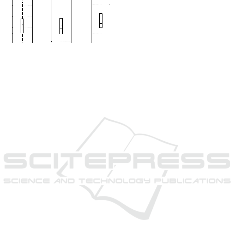
(a)
Age
30
35
40
45
50
55
60
(b)
Training
4
6
8
10
(c)
km in 2014
5k
10k
15k
Figure 1: Subject’s distribution concerning (a) age, (b) av-
erage weekly training time, and (c) overall cycling distance
in 2014.
with respect to the attainable simulation quality us-
ing the presented experimental setting. Underlying
measures here are 60 minutes Peak Power (PP60)
for performance, and Training Stress Score (TSS) for
strain. The PP60 is used because of the lack of physi-
ological parameters like blood lactate concentration,
˙
VO
2
max or similar conditioned by the data gather-
ing, but is found a useful measure for outdoor cy-
cling performance (Balmer et al., 2000; Tan and Aziz,
2005). Since solely values deduced from measured
values were available, we compared the RMSE fitting
quality of different TRIMP values, Skiba’s bike score
and TSS. Here, TSS reached best results, although all
measures were located in a very similar range.
Out of 52 cyclists that registered only 20 supplied
sufficient data for fitting, i.e., including both a value
for the strain metric and for the performance metric
and generating data using a power meter. Figure 1
shows the distribution of all 20 subjects concerning
age, average weekly training time and performed cy-
cling distance in 2014 per subject. All subjects had
been familiarized with the utilization of their pro-
vided data for research purposes and have been ac-
quaint about their self-responsibility in training and
data elicitation. Data privacy is ensured by design and
by pseudonymization.
3.2 Fitting Concept
In terms of adapting a performance model to a sub-
ject, the model’s parameter set has to be figured out.
A least squares approach is used to fit parameters to
given data as widely suggested, e.g., by (Busso et al.,
1997). In preliminary comparative studies we found
any state of the art Quasi-Newton method to show
similar or better performance than stochastic search
methods while being computationally less expensive.
One of the model parameters describes the con-
cept of an initial performance level which is mod-
eled by p
∗
in the Fitness-Fatigue model, while the
other parameters are time constants describing how
fast a subject adapts to strain. p
∗
represents the per-
formance level without any specific training. It is also
the level an athlete returns to after stopping training.
Usually, laboratory studies make a specified train-
ing plan compulsory for each subject and often last
between 4 to 60 weeks, cf. (Pfeiffer, 2008). Per-
formance is often tested every three to five weeks
(cf. (Hellard et al., 2006; Busso et al., 1991)). In
these plans, fluctuating strain is provided in order to
fit model parameters to the subject’s adaptability. Fur-
thermore, subjects are aware of their responsibility
and controlled by some training supervisor. Since the
idea of the traipor concept was to simulate or pre-
dict performance process without laboratory studies
and fixed training plans, such data can not be taken
as assured here. To deal with training data from non-
predefined workout and without a certain quality, a
special fitting concept is elaborated.
The therefore designed traipor concept for fitting
can be subdivided in two parts: 1. data cleansing, and
2. data grouping. After this concept of preparing data,
subject’s individual parameters are determined using
a least squares approach evaluated on training days
only. Following parameter fitting, a training plan can
be generated as described in (Schaefer et al., 2015)
regarding individual constraints.
3.2.1 Data Cleansing
Restricting the duration of training data to the cur-
rent and last year: As stated before, laboratory stud-
ies usually fit their models over a one to few month
period of time. These studies predefine a training plan
for subjects and can control the execution. Usually,
subjects can perform a variety of different load and
performance levels, whereby performance limits were
tested regularly. Since there is no supervision or con-
trol in this study, any performance development has to
be extracted from training data itself. A longer period
for fitting therefore is beneficial, since adaptability of
the human body to training can be mapped to the set
of system inherent variables. This is stated as general
adaptability to fitness and fatigue within the param-
eter set. But if the fitting period is too long, body
might have changed this adaptability over years and
react different to training.
Rejecting data which do not include both a value
for the strain metric and for the performance metric:
This step is necessary to avoid unusable data since
both values are inalienable.
3.2.2 Data Grouping
Group data sets according to the subjects specifica-
tion: Within each group, the highest performance
Training Simulation with Nothing but Training Data - Simulating Performance based on Training Data Without the Help of Performance
Diagnostics in a Laboratory
77
ttf tf tf
Strain (TSS)
Measured Performance
Assumption
TSS / PP60
Figure 2: Grouping of data. The highest performance value
of each group tf is chosen to replace other performance val-
ues within this time frame (dotted line).
value replaces all values inside this group. Consid-
ering that even ambitious sportsperson do not reach
their personal performance limit within each training,
using every single performance value in fitting might
lead to highly fluctuating performance in a short time.
Therefore, information is needed about the approx-
imate time frame in which the subject does usually
reach its performance limit, e.g., weekly, biweekly, or
monthly. This information was provided by the sub-
ject itself. The highest performance in this specific
time frame approximate the real performance limit
more accurate and therefore is chosen for all perfor-
mances within this period. An example is illustrated
in Figure 2. For the specified length of the time frame
tf, given data set excerpt is divided into three groups.
Strain performed within a training session is repre-
sented by rectangles. After identifying the highest
performance value, all other performance values are
substituted with the very same and depicted as dotted
lines.
Accumulate all strain data performed on one day:
To use just one single value of strain and performance
for each day, strain is accumulated if training was per-
formed on several occasions same-day. Performance
value remains at the maximum performance value de-
termined beforehand during grouping of data.
3.3 Experiments
We divided our experiments into three main parts:
1. Ability of the presented concept to improve fitting
quality for outdoor training data in general.
2. Comparison of results between this concept and
laboratory studies to prove usability.
3. Analysis of the underlying data in cases where fit-
ting does not reach a reliable accuracy.
When comparing our results to laboratory studies,
fitting correlation serves as reference value: In (Pfeif-
fer, 2008), results are evaluated using the intraclass
correlation coefficient r
ICC
in version of r
ICC
(1,1)
(one-way random, single measure) regarding (Shrout
and Fleiss, 1979). The study of (Busso et al., 1991)
uses the Pearson correlation coefficient r, and (Hel-
lard et al., 2006) and (Mujika et al., 1996) are using
the coefficient of determination r
2
. Accordingly, re-
sults from the described fitting concept are stated as
r
ICC
, r or r
2
value. Correlation measures are com-
puted between the simulated performance curve ac-
cording to estimated parameters from the fitting con-
cept, and measured performance values.
3.4 Statistical Analyses
Considering performance analyses, it is important to
know the accuracy of the fitting for a specific method.
The quality of a method is often given by the deviation
between a simulated curve compared to the measured
one.
Let n be the number of data points, x
i
the mea-
sured values with mean x and let y
i
be the simulated
values with mean y, i ∈ {1,2,...,n} . The absolute er-
ror is defined by e
i
= |x
i
−y
i
|. The sum of squares er-
ror (SSE) is defined by SSE =
∑
n
i=1
e
2
i
, while the total
sum of squares (SST) is given as SST =
∑
n
i=1
(x
i
−x)
2
.
A total sum of squares for the simulation is indicated
with SST
y
. The root-mean-square error (RMSE) is
defined by RMSE =
q
SSE
n
and serves as kind of a
standard deviation between the measured and the es-
timated curves.
Since different studies use different sta-
tistical measurements as described before,
these values were computed as well with
r =
∑
n
i=1
(x
i
− x) · (y
i
− y) / (
√
SST ·
p
SST
y
),
r
2
= 1 − SSE/SST, and r
ICC
= ICC(1,1) according
to (Shrout and Fleiss, 1979). In all of these corre-
lation measures, a correlation value of 1 indicates a
good correlation and values near 0 indicate a missing
correlation. A value near -1 in r or r
ICC
correlation
value implies a negative correlation respectively.
Regarding statistical measures such as r with time
series with within-series dependencies, some difficul-
ties have to be considered. With correlation coeffi-
cients, goodness of fit and accuracy can not be mod-
eled adequately, it does only model the time-series
behavior in general. A good correlation value is
achieved if the curve structure of measured perfor-
mance and simulated performance are similar to each
other independent of possible variation in range or
scaling. Furthermore, if the measured performance
is given by a straight line such that the total sum of
squares sums up to zero or some small value near
zero, r and r
2
are undefined or quite low even if
the simulated performance contains only small vari-
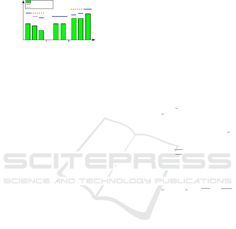
ances. Figure 3 shows an example where the r-value
is undefined and indicates no correlation whereas
icSPORTS 2016 - 4th International Congress on Sport Sciences Research and Technology Support
78
0 5 10 15 20 25 30
0
100
200
300
400
days
TSS / PP60
Strain (TSS)
Measured Performance
Simulation
Figure 3: Example where the fitting process results in a
small deviation, whereas the r-value is undefined.
Table 1: Comparison of the RMSE and r-value both as
mean, median and standard deviation with and without the
traipor concept.
raw data concept
RMSE
mean 35.77 14.13
median 40.59 12.07
std 18.27 6.43
r-value
mean 0.27 0.57
median 0.26 0.65
std 0.12 0.25
the simulated performance curve does not deviate
much (RMSE = 8.72) from the measured performance
curve.
Therefore, we consider the r-value as one exem-
plary correlation measure to analyze a possible gen-
eral similarity between the fitting and the measure-
ment. But for measuring the fitting quality itself, we
particularly consider the RMSE.
4 RESULTS
Following we prove that the concept is useful to im-
prove fitting quality for outdoor training, and is com-
parable to laboratory studies in some cases. Cases
were correlation can not reach such high values as in
laboratory studies are further analyzed in the end.
4.1 Usefulness of the Presented Concept
To prove that presented concept is able to improve fit-
ting quality for outdoor training data, Table 1 shows
the average, median and standard deviation of the
RMSE and r-value over all subjects for both cases,
the raw data and the preprocessed data according to
the traipor concept. While the error can be reduced
more than 50%, the correlation value doubles for the
processed data sets proving both, a better correlation
and smaller deviation compared to the highly fluctu-
ating raw data.
0 5 10 15 20
0
0.2
0.4
0.6
0.8
1
Fitting Correlation
r
ICC
r
r
2
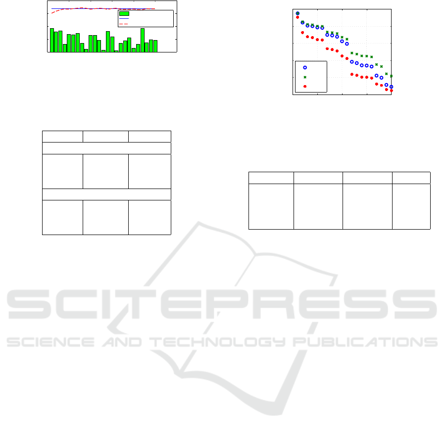
Figure 4: Correlation values of r
ICC
, r, and r
2
for all 20
subjects (sorted).
Table 2: Average r
ICC
-value, median and standard devia-
tion over the correlating amount of subjects for studies from
Pfeiffer and the traipor concept.
Pfeiffer 1 Pfeiffer 2 traipor
Subjects 3 3 11
Mean 0.67 0.28 0.75
Median 0.64 0.45 0.78
Std. 0.12 0.38 0.10
4.2 Comparison to Laboratory Studies
Training data used in this study was obtained with-
out any quality control. Therefore, we analyzed the
reachable correlation according to the correlation val-
ues r
ICC
,r, and r
2
for all single subjects. Figure 4
shows these correlation values for each subject, sorted
descending by the corresponding value. Notwith-
standing that these three values were sorted indepen-
dently of each other, all three measures indicate a
high fitting correlation for up to the same 11 sub-
jects. We therefore restricted the following compar-
isons to these subjects first. The remaining nine sub-
jects are analyzed more individually afterwards in
subsection 4.3.
The first comparison is made between the traipor
concept and two studies described in (Pfeiffer, 2008).
Table 2 shows average, median and standard devia-
tion computed for the intraclass correlation coefficient
r
ICC
for the correlating results. The mean and median
value conducted over the best 11 subjects indicates a
higher correlation than in results from (Pfeiffer, 2008)
and even standard deviation is much smaller.
Table 3 illustrates the comparison of the presented
method with a study from (Busso et al., 1991). Here,
results of the presented traipor concept reach similar
correlation in median as Busso’s laboratory study, but
seems to have more variation according to the stan-
dard deviation and the greater variation to the average
r-value. A restriction to eight subjects is able to reach
the same average correlation.
Regarding r
2
-value and the study from (Mujika
et al., 1996), Table 4 (left) indicates similar results:
Training Simulation with Nothing but Training Data - Simulating Performance based on Training Data Without the Help of Performance
Diagnostics in a Laboratory
79

Table 3: Average r-value, median and standard deviation
over the correlating amount of subjects for the study from
Busso and the traipor concept.
Busso traipor
Subjects 8 11 8
Mean 0.83 0.78 0.83
Median 0.81 0.80 0.82
Std. 0.06 0.09 0.07
Table 4: Average r
2
-value, median and standard deviation
over the correlating amount of subjects for studies from Mu-
jika and Hellard and the traipor concept.
Mujika Hellard traipor
Subjects 18 9 11 9 2
Mean 0.65 0.79 0.61 0.65 0.82
Median – 0.78 0.64 0.64 0.82
Std. 0.12 0.13 0.14 0.12 0.13
traipor concept’s average r
2
correlation regarding
nine subjects is stated in a similar range as the av-
erage correlation coefficient in Mujika’s study, for 11
subjects it is slightly below. Solely results of the study
from (Hellard et al., 2006) (Table 4, middle) achieve
an obvious better average correlation (0.79) than the
traipor concept which yields comparable results for
the best two subjects only. Depending on the particu-
lar study except for Hellard et al., data of between 8
and 11 subjects reached comparable correlations for
simulating performance.
4.3 Analysis of Lower Correlated Data
The remaining nine data sets where results were not
able to reach comparable correlation as in laboratory
studies are analyzed in more detail. These nine data
sets are therefore subdivided into groups with a sim-
ilar performance behavior. Since it was necessary
to exclude three data sets for comparison to Busso’s
study, these are analyzed first.
Two out of three subjects which are excluded for
comparison to Busso’s study are identically to the
subjects excluded for comparison to Mujika’s study.
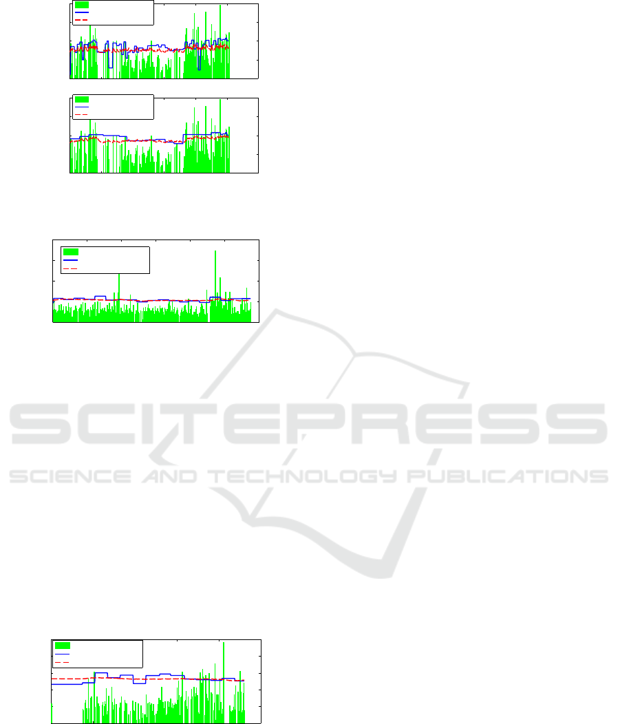
Exemplary, data of two of these subjects is illustrated
in Figure 5. Data of the third one shows a similar be-
havior as depicted in Figure 5a showing some huge
performance leaps which are not always reasonable
according to the underlying strain. As an example,
the performance gain between day 67 and day 118
based solely on the performance peak right before on
day 66. But with a training pause of over a month,
real performance would rather decrease than stay at
this higher level. Leaps like this are therefore ques-
tionable and a behavior like this is certainly not sim-
ulated by the model. Figure 5b shows a different be-
(a)
0 100 200 300 400 500 600
0
100
200
300
400
days
TSS / PP60
Strain (TSS)
Measured Performance
Simulation
(b)
0 50 100 150 200 250 300
0
100
200
300
400
days
TSS / PP60
Strain (TSS)
Measured Performance
Simulation
Figure 5: Exemplary subjects which has to be excluded for
the comparison with Busso.
havior: Here, performance does not change much at
all and varies around a mean performance value. As
explained in subsection 3.4, the r-value is often very
low when data is altering sparsely around its mean
value.
For a better overview, the remaining nine subjects
are numbered consecutively from 1 to 9.
Subjects 1-4: Regarding all 20 subjects, four of
them stated a weekly reaching of the individual per-
formance limit. But all of these four subjects are
inside the set of the excluded nine subjects. There-
fore, we analyzed correlation and fitting quality for
these subjects again, assuming a monthly reaching of
the performance limit. Table 5 shows the compar-
ison between assuming a weekly and monthly per-
formance limit for these subjects. Since the r-value
of one subject reaches only a significance-level of
p < 0.5% while the other three are significant at a
p < 0.01% level, correlation and error values are con-
sidered for three and four subjects respectively. Re-
garding three subjects, assuming the reaching of a
monthly performance limit improves the average cor-
relation from r = 0.42 up to r = 0.57 within these
subjects, while evaluating all four subjects shows an
average improvement from r = 0.4 to r = 0.47. Ex-
Table 5: Assuming a weekly or monthly reaching of the
individual performance limit regarding 4 or 3 specific sub-
jects.
4 Subjects 3 Subjects
weekly monthly weekly monthly
RMSE
mean 26.52 17.74 29.27 19.10
median 28.18 14.80 31.95 15.93
std 8.45 7.24 7.86 8.22
r-value
mean 0.40 0.47 0.42 0.57
median 0.40 0.55 0.44 0.58
std 0.07 0.22 0.08 0.05
icSPORTS 2016 - 4th International Congress on Sport Sciences Research and Technology Support
80
(a)
0 100 200 300 400 500 600
0
100
200
300
400
days
TSS / PP60
Strain (TSS)
Measured Performance
Simulation
(b)
0 100 200 300 400 500 600
0
100
200
300
400
days
TSS / PP60
Strain (TSS)
Measured Performance
Simulation
Figure 6: Example for a subject stating a weekly reaching
of the individual performance limit.
0 100 200 300 400 500 600
0
200
400
600
800
days
TSS / PP60
Strain (TSS)
Measured Performance
Simulation
Figure 7: Example without huge performance gain resulting
in a minor r-value.
emplary, Figure 6a shows a simulation with weekly
assumed performance limit while Figure 6b illustrates
the same dataset with a monthly assumed reaching of
the performance limit.
The remaining five subjects with a correlation
value of r < 0.6 can be classified into two classes:
Subjects 5 to 8 could not achieve any distinct per-
formance changes and varied around their average
performance as shown exemplary in Figure 7. This
problem has been explained before.
Subject 9: Data of the last subject again shows the
converse behavior including large unexplainable per-
formance leaps additional to some flat performance
in the end. The overall performance did not change
much over the whole time as shown in Figure 8.
0 100 200 300 400 500
0
100
200
300
400
500
days
TSS / PP60
Strain (TSS)
Measured Performance
Simulation
Figure 8: Example without huge performance gain but some
leaps in the middle resulting in a minor r-value.
4.4 Evaluation and Discussion
Considering the intraclass correlation, a high corre-
lation is accomplished with even better results than
those achieved in the corresponding laboratory stud-
ies from (Pfeiffer, 2008). Pfeiffer himself found that
results of his study 2 are inacceptable, but stated re-
sults from study 1 as good and very acceptable out-
comes. For up to eleven subjects, the traipor concept
reached higher correlation values than study 1.
Regarding the fitting correlation in comparison to
studies from (Busso et al., 1991) and (Mujika et al.,
1996), results implicate that the traipor concept is as
accurate as laboratory studies for 8 to 9 out of 20 sub-
jects, since average correlation values are stated in a
similar range. Fitting accuracy of the traipor concept
is only clearly inferior compared to (Hellard et al.,
2006). One reason for this might be because of dif-
ferent types of athletes. The study of (Hellard et al.,
2006) was performed for nine elite swimmers. (Mu-
jika et al., 1996) analyzed performance in swimming,
too, but regarding the considered studies, only Hellard
et al. explicitly state dealing with elite sportsperson.
Data of the traipor concept originates from ambitious
but non-professional sportsperson, in case of the re-
stricted data aged 34 to 49 years, whose fitness is cer-
tainly not comparable to elite swimmers. This differ-
ence regarding the subjects might be a reason for this
various correlation quality.
As stated before, the elaborated traipor concept
for fitting has some differences compared to labo-
ratory studies. These lead to few limitations which
might lessen the accuracy and correlation of fitting.
Even in this approach it is necessary for a suitable
fitting that the subject reaches its personal limit regu-
larly, e.g., weekly or monthly. Without reaching the
own individual limit, a realistic performance progress
is not possible using the traipor concept. Further-
more, an oscillating training strain might lead to an
inconvenient parameter set modeling a constant strain
located between both performance values. Regarding
correlation coefficients, the data grouping might lead
to straight line performances resulting in an undefined
r-value as explained in subsection 3.4. Additionally,
this procedure might result in unrealistically high per-
formance values during a training pause if computing
a monthly performance maximum includes both, the
training break and a high performance value achieved
before the rest. Despite the fitting on training days
only, some unrealistic performance changes may oc-
cur. These limitations are due to the unsupervised
and uncontrolled training without any specified per-
formance gain and the therefore constructed data pre-
processing.
Training Simulation with Nothing but Training Data - Simulating Performance based on Training Data Without the Help of Performance
Diagnostics in a Laboratory
81

5 CONCLUSION AND FUTURE
WORK
Compared to laboratory studies, the presented traipor
concept yields comparable results with similar fitting
accuracy using the Fitness-Fatigue model.
Since this model is based on a convolution with
an exponential function, a straight line as it results by
replacing all measurements within one period (e.g.,
month) by the maximum value can generally not be
approximated. Changing this concept should there-
fore be considered. Other approaches using differ-
ent filters should be analyzed. Using a moving maxi-
mum function might also reduce leaps between differ-
ent performance measurements. This way, unrealistic
performance values near to a training break might be
avoided or reduced at least.
Predicting future performance based on a given
training plan is an interesting application of train-
ing models, e.g., to generate training plans to reach
a certain goal. Using the described method, it is
possible to predict training effects for the upcoming
month with similar accuracy as achieved in fitting
(RMSE = 16.56). Even predicting six month into
the future yields acceptable results (RMSE = 20.62)
in all 11 subjects. Since in prediction preload plays
an important role (i.e., accumulated strain at T = 0)
special treatment of initial performance p
∗
was nec-
essary. Further research will be required to examine
the influence of preload as it should generally be con-
sidered in model identification.
Analysis of further performance metrics, espe-
cially for submaximal performances as these are more
common in non-athletes, would be promising by en-
abling the utilization of training models in mass sports
and training devices. To verify accuracy results, fur-
ther experiments with more subjects, even less ambi-
tious cyclists and additional laboratory control exper-
iments have to be conducted.
ACKNOWLEDGEMENT
This work was supported by a funding of the state
North Rhine-Westphalia, Germany.
REFERENCES
Balmer, J., Davison, R. R., and Bird, S. R. (2000). Peak
power predicts performance power during an outdoor
16.1-km cycling time trial. Medicine and Science in
Sports and exercise, 32(8):1485–1490.
Busso, T., Candau, R., and Lacour, J.-R. (1994). Fatigue
and fitness modelled from the effects of training on
performance. European journal of applied physiology
and occupational physiology, 69(1):50–54.
Busso, T., Carasso, C., and Lacour, J.-R. (1991). Adequacy
of a systems structure in the modeling of training ef-
fects on performance. Journal of Applied Physiology,
71(5):2044–2049.
Busso, T., Denis, C., Bonnefoy, R., Geyssant, A., and La-
cour, J.-R. (1997). Modeling of adaptations to phys-
ical training by using a recursive least squares algo-
rithm. Journal of applied physiology, 82(5):1685–
1693.
Calvert, T. W., Banister, E. W., Savage, M. V., and Bach, T.
(1976). A systems model of the effects of training on
physical performance. IEEE Transactions on Systems,
Man and Cybernetics, (2):94–102.
Hellard, P., Avalos, M., Lacoste, L., Barale, F., Chatard, J.-
C., and Millet, G. P. (2006). Assessing the limitations
of the banister model in monitoring training. Journal
of sports sciences, 24(05):509–520.
Krebs, P. and Duncan, D. T. (2015). Health app use among
us mobile phone owners: A national survey. JMIR
mHealth and uHealth, 3(4).
Lee, J.-M., Kim, Y., and Welk, G. J. (2014). Validity of
consumer-based physical activity monitors. Med Sci
Sports Exerc, 46(9):1840–8.
Mujika, I., Busso, T., Lacoste, L., Barale, F., Geyssant, A.,
and Chatard, J.-C. (1996). Modeled responses to train-
ing and taper in competitive swimmers. Medicine and
science in sports and exercise, 28(2):251–258.
Perl, J. (2000). Antagonistic adaptation systems: An exam-
ple of how to improve understanding and simulating
complex system behaviour by use of meta-models and
on line-simulation. 16th IMACS Congress.
Pfeiffer, M. (2008). Modeling the relationship between
training and performance-a comparison of two antag-
onistic concepts. International journal of computer
science in sport, 7(2):13–32.
Schaefer, D., Asteroth, A., and Ludwig, M. (2015). Train-
ing plan evolution based on training models. In
2015 International Symposium on Innovation in In-
telligent SysTems and Applications (INISTA) Proceed-
ings, pages 141–148.
Shrout, P. E. and Fleiss, J. L. (1979). Intraclass correla-
tions: uses in assessing rater reliability. Psychological
bulletin, 86(2):420.
Tan, F. H. and Aziz, A. R. (2005). Reproducibility of out-
door flat and uphill cycling time trials and their per-
formance correlates with peak power output in moder-
ately trained cyclists. J Sports Sci Med, 4(3):278–284.
Yang, R., Shin, E., Newman, M. W., and Ackerman, M. S.
(2015). When fitness trackers don’t ’fit’: End-user dif-
ficulties in the assessment of personal tracking device
accuracy. In Proceedings of the 2015 ACM Interna-
tional Joint Conference on Pervasive and Ubiquitous
Computing, UbiComp ’15, pages 623–634, New York,
NY, USA. ACM.
icSPORTS 2016 - 4th International Congress on Sport Sciences Research and Technology Support
82
