
Dealing with Groups of Actions
in Multiagent Markov Decision Processes
Guillaume Debras
1,2,3
, Abdel-Illah Mouaddib
1
, Laurent Jean Pierre
1
and Simon Le Gloannec
2
1
Universit
´
e de Caen - GREYC, Caen, France
2
Cordon Electronics DS2i, Val-de-Reuil, France
3
Airbus Defence and Space,
´
Elancourt, France
Keywords:
Markov Decision Processes, MultiAgent Decision Making, Game Theory and Applications, Robotic Appli-
cation.
Abstract:
Multiagent Markov Decision Processes (MMDPs) provide a useful framework for multiagent decision making.
Finding solutions to large-scale problems or with a large number of agents however, has been proven to
be computationally hard. In this paper, we adapt H-(PO)MDPs to multi-agent settings by proposing a new
approach using action groups to decompose an initial MMDP into a set of dependent Sub-MMDPs where
each action group is assigned a corresponding Sub-MMDP. Sub-MMDPs are then solved using a parallel
Bellman backup to derive local policies which are synchronized by propagating local results and updating the
value functions locally and globally to take the dependencies into account. This decomposition allows, for
example, specific aggregation for each sub-MMDP, which we adapt by using a novel value function update.
Experimental evaluations have been developed and applied to real robotic platforms showing promising results
and validating our techniques.
1 INTRODUCTION
Over the last decade, the improvement of small sen-
sors and mobility performance has allowed us to make
smaller and cheaper robots with better capabilities, be
it cameras, movement detectors, or hardware. This
opens the door to the use of teams of multiple robots
for a wide range of applications, including surveil-
lance, area recognition, human assistance, etc. We
are however still unable to provide software for mak-
ing those groups of agents (partially) autonomous due
to complexity problems. In fact, the modelling of the
world, the management of its dynamics, and the man-
agement of the possible interactions between agents
make the problem of action planning extremely com-
plex.
The MMDP model is a mathematical tool used
to formalize such decision planning problems with
stochastic transitions and multiple agents. The com-
plexity of solving such problems is known as P-
Complete (Bernstein et al., 2000) (Goldman and Zil-
berstein, 2004).
In this paper, we solve a problem composed of
multiple tasks without making assumptions on the
transitions (Becker et al., 2004)(Parr, 1998) or on hav-
ing a sparse matrix (Melo and Veloso, 2009).
We consider these hypotheses useful and manda-
tory for solving an MMDP in a reasonable time, but
they are too strict to be used easily on a general prob-
lem. We split the problem into smaller problems
using action space decomposition without a loss of
quality. We do not explicitly consider time (Messias
et al., 2013) or communications (Xuan et al., 2001)
but our model could be easily adapted to do so. Like-
wise, recent work on the use of the aggregate effect
of other agents (Claes et al., 2015) (Matignon et al.,
2012) instead of the outcome of every agents could be
adapted to each smaller problems to further improve
the boundaries of the initial problem. Many existing
approaches have been developed using space and pol-
icy decomposition, but little attention has been paid to
the use of action space decomposition (Pineau et al.,
2001). This decomposition allows us to split a com-
plex problem into sub-problems by forming action
groups. Such groups are motivated by many prob-
lem classes such as task, role and mission allocation
problems. We are thus working on a subdivision of
the general MMDP into smaller MMDPs, often re-
ferred to in the following as the Initial-MMDP and
its Sub-MMDPs, using action and state variables. We
Debras, G., Mouaddib, A-I., Pierre, L. and Gloannec, S.
Dealing With Groups of Actions in Multiagent Markov Decision Processes.
DOI: 10.5220/0006048000490058
In Proceedings of the 8th International Joint Conference on Computational Intelligence (IJCCI 2016) - Volume 1: ECTA, pages 49-58
ISBN: 978-989-758-201-1
Copyright
c
2016 by SCITEPRESS – Science and Technology Publications, Lda. All rights reser ved
49

solve in parallel all of the sub-problems with suitably
adapted synchronization mechanisms to find realistic
solutions. This allows us to consider problems with
no (in)dependent links between these sub-problems.
Furthermore this subdivision allows us to use other
techniques, such as aggregation, to decrease the solv-
ing time and get near optimal policies.
2 BACKGROUND
2.1 MMDPs
MMDPs are an extension of MDPs (Boutilier,
1996)(Boutilier, 1999) for multiagent problems, and a
particular case of Dec-MDPs (Bernstein et al., 2000)
where the environment is fully observable by each
agent of the system. An MMDP is defined by a tu-
ple hI,S,{A
i
},T ,R, hi, where:
• I is a finite set of agents;
• S is a finite set of states;
• A
i
is a finite set of actions for each agent i, with
A = ×
i
A
i
, the set of joint actions, where × is the
Cartesian product operator;
• T is a state transition probability function, T : S ×
A × S → [0, 1], T (s, a, s
0
) being the probability of
the environment transitioning to state s
0
given the
current state s and the joint action a;
• R is a global reward function: R : S × A → R,
R(s, a) being the immediate reward received by
the system for performing the joint action a in
state s;
• h is the number of steps until the problem termi-
nates, called the horizon.
2.2 Factored-MMDPs
Factored-MMDPs (Guestrin et al., 2002) are a sub-
set of MMDPs where the state is partitioned into
variables, or factors: S = X
1
× ... × X
|X|
where X =
{X
1
, ..., X
|X|
} is the set of variables. A state cor-
responds to an assignment of values of all factors
s = hx
1
, ..., x
|X|
i.
In a factored MMDP, the transition and reward
functions can be represented compactly by exploit-
ing conditional independence between variables and
additive separability of the reward function.
2.3 Hierarchical POMDP
The idea behind the Hierarchical Partially Observable
Markov Decision Process (H-POMDP) (Pineau et al.,
2001) is to partition the action space; the state space
is not necessarilly fully observable and thus can’t be
partitioned directly. The hierarchy is supposed given
by a designer and takes into account the structural
prior knowledge about the problem. An action hier-
archy can be represented as a tree where each leaf is
labeled by an action from the target POMDP prob-
lem’s action set. The tree is composed of leaves,
which are real actions, or ”primitive actions”, and in-
ternal nodes, which are ”abstract actions”. In order
to reduce the solving process, the action hierarchy
translates the original full POMDP into a collection
of smaller POMDPs defining a complete policy.
Figure 1: General Form Action Hierarchy.
3 OUR APPROACH
(Pineau et al., 2001) suppose with the H-POMDP ap-
proach, that a separation of actions leads to a wide
range of possible improvements on sub-parts of the
problem. This work, however, was only done in the
mono-agent case, and its application to a multiagent
one is far from simple.
Their resolution of the problem permits some
steps to be simplified as they consider that there is
a unique agent modifying the environment. In a mul-
tiagent situation, this assertion is invalid. We adapt
their concepts to Multiagent MDPs, and propose a
new way of solving such a problem by making groups
of actions that allow the use of meaningful improve-
ments such as aggregation generated by the consid-
ered actions.
To illustrate the model, we introduce a factored
safety surveillance (FSS) problem as a running exam-
ple. It formalizes a team of n robots that have to move
between r rooms, separated or not by d doors, with
the objective of making each room safe. A state in the
FSS problem is an assignment of the position of each
agent, the state of each door, and the safety level of
each room.
Figure 2 represents the problem with n = 2, r = 4
and d = 1. At each time step, each agent i can choose
ECTA 2016 - 8th International Conference on Evolutionary Computation Theory and Applications
50
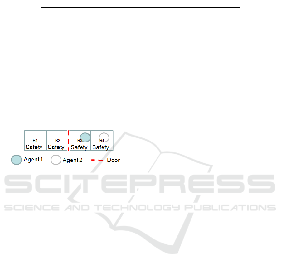
Table 1: Reduced set of states for each sub-problem for a (n; r; d) = (2; 4; 1) FSS problem.
JointAction StatesForm
RR RN NR [R1 R2O R2C R3 R4]
2
LL LN NL [R1 R2 R3O R3C R4]
2
NO ON OO OC CO CC CN NC [R2O R2C R3O R3C]
2
NS SN SS [R1 R2 R3 R4]
2
∗ [S N]
4
RO OR LO OL RC CR LC CL RL LR [R1 R2O R2C R3O R3C R4]
2
RS SR [R1 R2O R2C R3 R4]
2
∗ [S N]
4
LS SL [R1 R2 R3O R3C R4]
2
∗ [S N]
4
OS SO CS SC NN [R1 R2O R2C R3O R3C R4]
2
∗ [S N]
4
to move left or right between rooms (L,R), open or
close the door (O,C), make its room safe (S) or do
nothing (N). The advantage of this small example is
its strong coupling making most of the states interac-
tive and thus difficult to solve. Without loss of gener-
icness and for reasoning simplicity, we assume that
the environment is modified by the agents only.
Figure 2: Factored safety surveillance problem, with two
agents in a four room environment.
Our objective is to produce, from the initial prob-
lem, a set of sub-problems that are created using the
factored set of states S = X
1
×X
2
×... × X
n
by consid-
ering that ∀a ∈ A, X
a
= {X
i
|X
i
∈ X and X
i
is affected
by a}.
X
i
is affected by a if ∀s = (x
1
, x
2
, ..., x
n
) ∈ S, @s
0
=
(x
0
1
, x
0
2
, ...x
0
n
) ∈ S, s.t. T (s, a, s
0
) 6= 0 and x
k
6= x
0
k
.
In other words, if we represent a state as (X
1
= cur-
rent position, X
2
= safety of room1, etc.), a movement
action can (possibly) change the current position, but
can’t change the safety of a room. For a movement
action, we therefore consider that the position is af-
fected whereas the room safety is not.
By following this procedure, we can automatically
create every group G
S
i
containing every action that
affects the elements of S
i
.
4 FROM INITIAL- TO
SUB-MMDPs
We consider a factored initial MMDP, named Initial-
MMDP. We assume that we obtain an action decom-
position with p groups: G = hG
1
, ..., G
p
i with
S
i
G
i
=
A using the principles presented above. An action can
appear in multiple groups G
i
, however when those
groups are used to solve the problem, the action will
be processed multiple times. Unlike the H-POMDP
case (Pineau et al., 2001) we cannot assert an ac-
tion hierarchy because of the management of multi-
ple agents. A hierarchy based on the joint actions
could be made, but it is not discussed here. Using the
Initial-MMDP and each action group, we will create
Sub-MMDPs defined as a tuple hI, S
0
, A
0
, P
0
, R
0
, H
0
i:
• I is the number of agents of the Initial-MMDP;
• A
0
is the set of joint-actions considered in the ac-
tion group G
i
;
• S
0
is the factored set of joint states consisting of a
restriction of the Initial-MMDP; this restriction is
further explained in 4.1.2;
• P
0
: S
0
× A
0
× S
0
→ [0, 1] is the transition function
reduced to the working sets; R
0
: S
0
× A
0
→ ℜ the
immediate reward received by the system for be-
ing in state s and performing the joint action a;
• H
0
is the horizon.
We are inspired by the idea that to solve a complex
task, we do not need to be omniscient or omnipotent,
we just need to be able to process the available infor-
mation and do what is needed at the right moment.
In our example, the safety of the rooms has an im-
pact on the need to move, as it is the goal of the agent,
but is irrelevant to us while moving We therefore sep-
arate the actions into groups by examining only the
state variables which impact them. We use the follow-
ing form for the set of states: [AB]
i
∗ [CD]
j
will con-
tain every joint state that can be formed using i vari-
ables of [AB] and j variables of [CD]. In our example,
this gives the decomposition presented in the left col-
umn of 1. For example, [R1R2]
2
represents the states
for each agent, a joint state being R2R2. A likely pos-
sible instance of [R1R2]
2
∗ [SN]
2
is R2R1NS which
represents agent 1 in Room2, agent 2 in Room1, with
Room1 unsecured and Room2 secured.
Dealing With Groups of Actions in Multiagent Markov Decision Processes
51

4.1 Generation of the Sub-MMDPs
4.1.1 Problem Statement
The decomposition of the Initial-MMDP into multi-
ple Sub-MMDPs offers several possibilities. This de-
composition, which amounts to dividing the transition
table between each action group, generates no infor-
mation loss and gives us the ability to regenerate the
Initial-MMDP from the Sub-MMDPs.
The initial problem is, however, hard to solve, as
we are forced to take into account all combinations
of states and actions. We can simplify the problem
by considering each individual Sub-MMDP. We can
reduce the state set (as some states are not affected
by that action group) and find local policies. Then by
synchronizing the different Sub-MMDPs, we can find
a solution to the initial problem.
We define synchronization as the propagation of
each Sub-MMDP’s information. It mostly consists
of transferring the information from the sub-problems
to the initial problem and vice-versa. This separation
gives many benefits, such as reduced processing time
(at the potential cost of some information loss) if we
use aggregation techniques.
4.1.2 Definition of the Reduced Sub-MMDP
State Set
We consider that a state that we can neither leave, nor
reach with an action in A
0
is irrelevant for the con-
sidered Sub-MMDP. We can therefore restrict the set
of states S
0
in the Sub-MMDP to {s ∈ S|∃s
0
∈ S, a ∈
A
0
, P
0
(s, a, s
0
) > 0}. Note that S is still
S
i
S
0
i
.
4.1.3 A Possible Improvement: Aggregation
By creating the groups as presented in 3 and the sets
by following the restrictions given above, we obtain
different Sub-MMDPs with restricted sub-sets of the
Initial-MMDP.
A human is capable of performing a wide range
of actions, but will only use a sub-set for a given task;
cooking skills are not usually useful whilst driving for
example. Even when multitasking, unnecessary infor-
mation and actions will be filtered out.
We can apply this human-like reasoning to
MMDPs, as we have a sub-set of actions in our Sub-
MMDPs that do not use every variable composing the
states. We are thus able to independently aggregate
the sets of each problem. These aggregations improve
each Sub-MMDP independently and need to be ad-
dressed during synchronizations to take dependencies
between Sub-MMDPs into account and allow a near
optimal overall policy to be obtained.
The aggregation can be seen as the deletion of at
least one variable, X
i
, or of some instantiations of a
variable, x
i
from the state s. Using 3, we obtained
groups of actions that work on the same variables X
i
.
By removing non-influential variables from the con-
sidered state, we aggregate the states and are able to
work on smaller sets.
We apply the aggregation process to generate
the set of states for the action “go right”, R, in our
example (this process being the same for every
action) as follows:
Performing action R, going from a room to the one
on its right, in any state, does not modify informa-
tion about the safety of a room. More formally:
∀s = {pos, state
D
, sa f e
R1
, sa f e
R2
, sa f e
R3
, sa f e
R4
} ∈
S, @s
0
= {pos
0
, state
0
D
, sa f e
0
R1
, sa f e
0
R2
, sa f e
0
R3
, sa f e
0
R4
}
∈ S s.t. ∃i ∈ {1,..,4}, sa f e
R
i
6= sa f e
0
R
i
and
T (s, R, s
0
) 6= 0. We can thus remove the variables
“sa f e
Ri
” from every state of the current set.
Conversely, although in rooms R1, R3 and R4 the
result of going right is not affected by whether the
door is open or closed, in R2, if the door is closed the
agent will stay in that room, but if the door is open it
will go to room R3. The state of the door is hence in-
fluential and should be considered in the sets of vari-
ables. The set of influential states for the action R is
therefore {R
1
, R
2
O, R
2
C, R
3
, R
4
} where, for example,
R
2
O means “Room 2, Door open”.
By doing the same for every action, we obtain the
sets of states used by each action. In an MMDP we
consider joint-actions and we therefore need to com-
pose these sets for every agent considered. The ag-
gregation on our FSS example is shown in 1.
4.2 Resolution
Solving an MMDP means finding the best action
for each state in the set of states. Solving a Sub-
MMDP will thus give us the best action (according
to this Sub-MMDP) for each state in the reduced set
of states. Note that this action is chosen according
to the local model and is therefore optimal for the
sub-problem only; the optimal action for the Initial-
MMDP, which takes into account every detail could
be different.
Without aggregration, the best action chosen by
comparing the local Sub-MMDPs, will be the best
action for the Initial-MMDP. If aggregation is used,
however, the loss of information means that the best
action chosen from the aggregated sub-MMDPs is
not necessarily the optimal solution for the Initial-
MMDP.
Contrary to a wide range of work using decompo-
sition of a problem into sub-problems, we do not con-
ECTA 2016 - 8th International Conference on Evolutionary Computation Theory and Applications
52

Figure 3: Problem Resolution.
sider that there are (in)dependent links between each
Sub-MMDP. Thus we cannot solve them separately,
and we need to synchronize them to be able to com-
pare their results. To this end, resolution, as depicted
in 3, is based on a series of parallel backups followed
by synchronization. We consider that there are two
types of synchronization:
• Sync
Result
is the process of computing the best
global action of the initial-MMDP from the local
best actions of the Sub-MMDPs;
• Sync
Subs
consists of locally propagating the ex-
pected rewards of the best global action generated
by the Sync
Result
process.
Both synchronizations are only applied to relevant
Sub-MMDPs, i.e. ones whose states’ variables are
affected by the global action. The following sections
describe the synchronization processes.
4.3 Sync
Result
Sync
Result
links the Sub-MMDP set of states S
0
with
other sub-problems in order to work on the same set of
variables X
R
. Going back from S
0
to the initial set of
states S of the Initial-MMDP is possible in every case.
By doing this, we can transfer the information, such
as the states, expected reward or the action dictated
by the policy, from one problem to another. More
formally, we can define X
R
and S
R
as follows:
• X
a
, X
b
are the sets of variables of Sub-MMDP a
and b respectively;
• S
0
a
= ×
X
i
∈X
a
(X
i
), S
0
b
= ×
X
j
∈X
b
(X
j
) are the sets of
states;
• X
R
= X
a
S
X
b
;
• S
R
= ×
X
i
∈X
R
(X
i
).
We also define
• the projection s
0
a
of the state s ∈ S
R
on S
0
a
: s
0
a
=
s.X
a
s.t. s
0
a
∈ S
0
a
;
• the policy: π
S
0
a
(s ∈ S
R
) = π
S
0
a
(s.X
a
).
A brief example:
• X
a
= {A, B,C}, X
b
= {C, D, E};
• S
0
a
= A × B ×C, S
0
b
= C × D × E;
• X
R
= {A, B,C, D, E}, S
R
= A × B ×C ×D × E;
• s = (a, b, c, d, e) ∈ S
R
projected on S
0
a
: s.X
a
=
(a, b, c).
We can then compare the local policies and deter-
mine π
S
R
: ∀s ∈ S
R
,V
π
S
R
(s) = max(V
π
S
0
a
(s),V
π
S
0
b
(s))
where V
π
S
0
i
(s) = V
π
S
0
i
(s.X
i
).
The resolution is thus decomposed into a Bellman
Backup on all Sub-MMDPs, which let us process π
S
0
i
for each Sub-MMDP i, then compare each obtained
π
S
0
i
to find a solution for the initial problem π
S
, and
finally to send the resulting information to every sub
problem. We can then repeat the same process. To
solve the system we use dynamic programming (Bell-
man, 1954).
4.4 Sync
Subs
Sync
Subs
propagates π
S
R
to every sub problem. In
order to manage the synchronization, we can con-
sider that the variables X
i
are grouped in an inter-
act, X
interact
= X
a
T
X
b
, and a normal set, X
normal
=
X
a
S
X
b
− X
interact
(Witwicki and Durfee, 2010). A
variable is in the interact set if there are at least two
sub-problems where this variable is influential. It is
possible to create such a set for every pair of sub-
problems or for the entire set of sub-problems de-
pending on the synchronization process we apply.
When the interact variables are modified, Sync
Subs
should be performed. More formally speaking: ∀s ∈
S
R
and a global action a = π
S
R
(s), we propagate
V
π
S
R
(s) to the relevant set S
0
i
of the Sub-MMDPs. As
each Sub-MMDP can observe variables modified by
the others, the processing and synchronization of all
the Sub-MMDPs must be carried out at the same time,
i.e. during same time interval. The synchronization is
Dealing With Groups of Actions in Multiagent Markov Decision Processes
53

done using the expected reward as a vector of com-
munication following this formula:
• ∀s ∈ S
R
, E[R
S
0
i
(s)] =
∑
s
0
=s.X
i
E[R(s
0
)]
|{s
0
,s.t. s
0
=s.X
i
}|
.
4.5 Sub-MMDP Synchronization with
Aggregation
This step propagates the results of each Sub-MMDP
to the other Sub-MMDPs. This corresponds to an up-
date of the value function of each Sub-MMDP based
on the results of the Bellman backup.
We consider a set of p states S
up
= {s
u1
, . . . , s
up
}
and its aggregated corresponding state s
agg
∈ S
agg
; the
corresponding value functions V
π
(s
t
u1
), . . . ,V
π
(s
t
up
) at
time t, giving the following update formulae:
∀s
agg
∈ S
agg
,V
π
(s
t
agg
) = max(V
π
(s
t−1
agg
), max
j
{
V
π
(s
t−1
u j
)
p
}
∀s
up
∈ S
up
,V
π
(s
t
up
) = max(V
π
(s
t−1
agg
),V
π
(s
t−1
up
))
These equations allow us to synchronize the set of
different sub-problems with different sets of variables
X
i
. This means that, instead of comparing each ac-
tion on every state (112 comparisons for our running
example with one agent), we would reduce the com-
parisons to the relevant states (23 comparisons). The
cost of synchronization, which mainly consists of ad-
ditions, does not outweigh this gain.
5 FROM SUB-MMDPs TO MMDP
The resolution of each Sub-MMDP
hI, S
0
, A
0
, P
0
, R
0
, H
0
i gives us the best joint-action
of its action group for each of its states. We
thus solve each Sub-MMDP using the following
value function: V
π
(s
t
) = E[
∑
h−1
t=0
γ
t
R(
−→
a
t
, s
t
)|π] with
−→
a
t
= π(s
t
.X
0
)
The action groups between them cover every
action of the Initial-MMDP, and the decomposition
of the states previously described does not prune any
state from which we can perform at least one action.
Resolving the initial problem is therefore the same
as finding the best joint-action - among all sets of
joint-actions - for each state - among all sets of states,
equivalent to using the following value function:
∀s
t
∈ S,V
π
Initial
(s
t
) = E[
h−1
∑
t=0
γ
t
max
Subs
(R
0
(
−→
a
t
, s
t
))]
with
−→
a
t
= π(s
t
.X
0
) and R
0
the reward function of the
Sub-MMDP.
We present in the following an algorithm to solve
the FSS problem. We note Sync
S
B
S
A
: S
0
S
A
7→ P (S
0
S
B
)
the function which returns the set of states S
B
of the
problem B corresponding to a state s of the problem
A: Sync
S
B
S
A
(s) = {s.X
S
B
}
s∈S
A
. A and B. Reference to
the initial is denoted by init and a sub problem by
sub.
Require:
1: h = 0
2: EF ={s|R(s) > 0}
3: P
sub
(s) = {s
2
|∃s
0
∈ Sync
sub
(s), s
2
∈
previousState
sub
(s
0
)} with s
0
∈ Sync
sub
(s)
4: while h < H do
5: for all sub ∈ set of sub-Problems do
6: EF
sub
= ∪
s∈EF
P
sub
(s)
7: for all s
0
∈ EF
sub
do
8: V
0
h
(s
0
) = E(V (s)|s
0
∈ Sync
sub
init
(s))
9: end for
10: for all s
2
∈ EF
sub
do
11: for all a ∈ A
0
sub
do
12: V
0
h+1
(s
2
, a)=cost(a)+γΣ
s
0
T (s
2
, a, s
0
)V
0
h
(s
0
)
13: end for
14: V
0
h+1
(s
2
) = max
a
V
0
h+1
(s
2
, a)
15: Π
0
(s
2
) = argmax
a
V
0
(s
2
, a)
16: end for
17: for all s ∈ Sync
init
sub
(s
2
), s
2
∈ EF
sub
do
18: V
sub
(s) = V
0
h+1
(s
2
)|s
2
= Sync
sub
init
(s)
19: Π
sub
(s) = Π
0
(s
2
)
20: EF = EF
S
{s}
21: end for
22: end for
23: V (s) = max
sub
V
sub
(s)
24: Π(s) = argmax
a
Π
0
(s, a)
25: end while
6 COMPLEXITY
The complexity of a MMDP is in the or-
der of magnitude of (|A|.|S|)
h
(Papadimitriou
and Tsitsiklis, 1987) (Littman et al., 1995),
our approach is in MAX
iingroups(G)
(|Ai|.|Si|)
h
+
complexityo f synchronization which is in the order of
h.|S|.|G|
2
.
Termination of the approach is guaranteed by the ter-
mination of MMDP solving: our approach is based
on a series of parallel sub-MMDP solving followed
by synchronization. Synchronization being done by
comparing the different groups results.
ECTA 2016 - 8th International Conference on Evolutionary Computation Theory and Applications
54
7 EXPERIMENTAL RESULTS
We consider factored safety surveillance prob-
lems with 2 agents, 1 to 2 doors and 3 to
6 rooms. The actions considered are Nothing,
MovingRight, MovingLe f t, OpenDoor, CloseDoor,
MakeRoomSa f e, with costs of 0,5,5,3,3 and 10 re-
spectively, the final states reward a vast amount
(1000). The sub-problems are defined using the
groups presented in 1. We solve each of those prob-
lems using an MMDP approach, with and without us-
ing groups. We consider in the following that “using
groups” is equivalent to “using aggregation”.
There is a non-reversible action (that of securing a
room), which allows us to prune a branch of the tran-
sition tree when no aggregation is made, as we can
assume that the agents will stop when the specified
rooms have been secured, and will not need to verify
the others. Using aggregation, on the other hand, we
lose information on the states, which does not permit
us to take the same shortcut. To be able to compare
both approaches in terms of solving time and policies,
we therefore need to consider that all rooms must be
secured before the agents stop. In each example, we
therefore consider a unique final state where all rooms
are secured and both agents stop in room 1. We do not
explicitly consider an intial state as the policy pro-
cessed will give plans for every possible state.
We already know that MMDPs can be solved op-
timally using the state of the art techniques (i.e. basic
value iterations). We therefore use this for both prob-
lems. The case where we do not consider groups of
actions gives us the optimal policy of the problem and
can be used as a reference to compare the results using
groups of actions.
For each case, we compare the average time to
solve the instance with and without groups, the num-
ber of states with positive rewards and the rewards
given by the computed policies for each horizon.
The experiments were conducted using a mono-
core at 2.4Ghz and 16Gb DDR3. Note that the
decomposition into sub-problems allows for parallel
solving using multi-cores (one for each sub in the best
case), but to be able to compare on a par with the basic
resolution we do not present those results here.
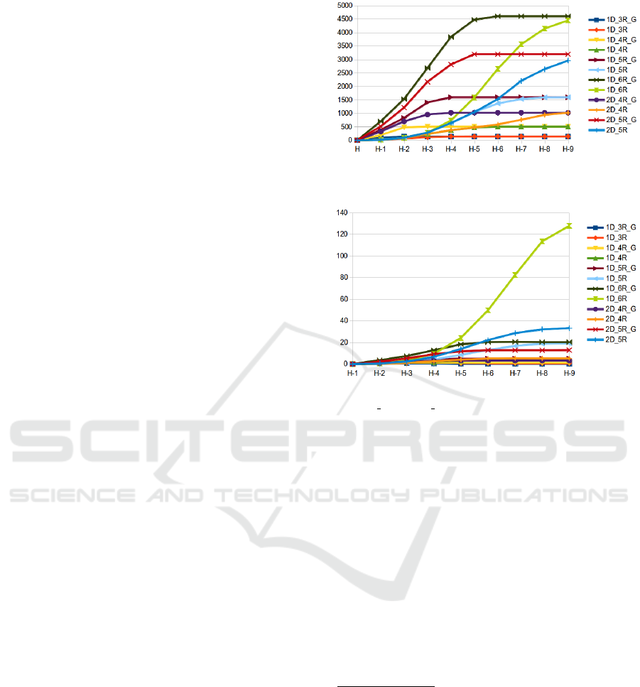
7.1 Performance
We hoped to show a possible gain in computation
time and space using our approach. One drawback
of our method appears to be the steeply rising num-
ber of Final States per Horizon at each step when us-
ing groups (see 4). The use of aggregation blurs the
boundaries among sub-problems and a state in a spe-
Figure 4: Average number of positive reward Final States
per Horizon.
Figure 5: Average solving time (sec) for the
XDoors YRooms( Group) instance per Horizon.
cific sub-problem (such as the position of the agents)
can be equivalent to several hundreds of states in an-
other sub-problem or in the initial problem where we
consider other variables such as room safety as well
as the agents’ position. We therefore expand the set
of reachable states very quickly. Despite this rapid
expansion, the resolution time is still much faster than
that of the standard solution due to the use of aggrega-
tion. 5 shows a significant gain in computation time,
directly resulting from the state space reduction re-
sulting from the use of aggregation.
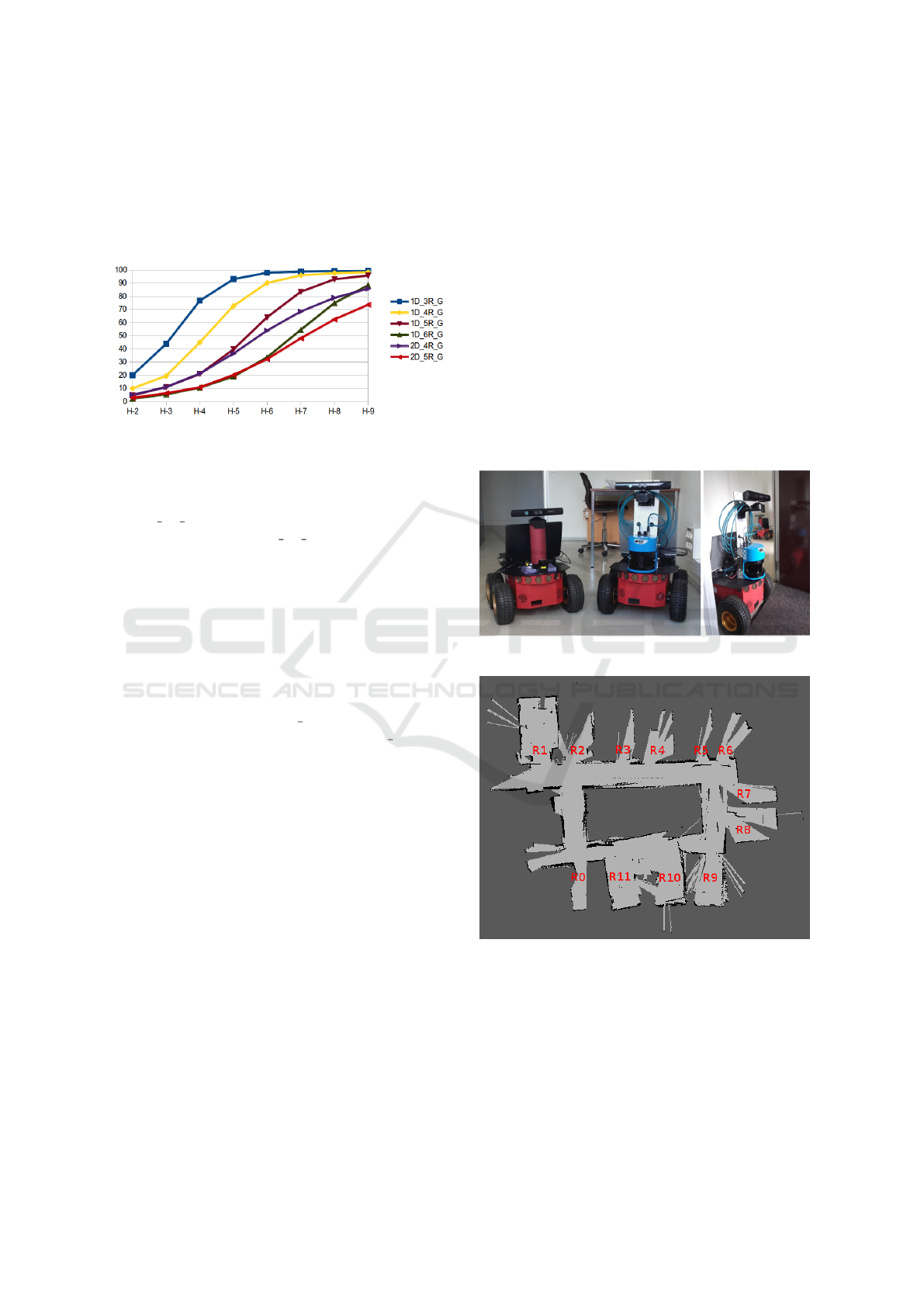
7.2 Solution Quality
6 shows us the comparison of:
∑
s∈FinalStates
(E[R(s)])
|FinalStates|
computed for the optimal case
(without groups) and the case using groups (and ag-
gregation).
Due to the process of aggregating and decompos-
ing states based on the variables X
i
, we find in the
policy using groups a lot of actions for states that are
not considered in the optimal policy. This particularly
shows in 4 for short horizons where the resolution not
using groups slowly expands its wave of states with
positive expected rewards. This explains the relatively
low rewards on shorter horizons in comparison to the
optimal case (without groups) shown in 6. The longer
the horizon, the better the results. Without groups, the
Dealing With Groups of Actions in Multiagent Markov Decision Processes
55
optimal policy reaches more states after each horizon,
and with groups, the synchronizations propagate the
expected rewards to the different sub-problems. The
policies obtained using groups are close to optimal, in
terms of actions chosen for each state, and in terms of
expected rewards on longer horizons.
Figure 6: Percentage of the optimal value per Horizon.
We can see that the error decreases the longer the
horizon and for large problems we need longer hori-
zons to attain a high solution quality. For example, in
the 1D 3R G problem we attain the optimal policy at
horizon 9 while for the 2D 5R G, we attain only 73%
of the optimal solution. In general, when considering
an infinite horizon, our approach will be faster to
show near-optimal solutions. The infinite horizon
consideration is however left for future works.
We note some drawbacks of the method that are
not shown in these results:
• The sub problems being different in term of num-
ber of states, the chosen joint action of the poli-
cies are sometimes Right Open in a state where
the door is already open, instead of Right Nothing
as in the optimal case. It is explained by the way
we manage and propagate the rewards on the sub
problems; we consider averages on the number of
states, and thus end with cases where performing
a useless action on a sub problem is better than
doing nothing on another;
• When the final states’ rewards are not high
enough, the aggregation process can not propa-
gate enough rewards to let the sub-problems be
solvable, and no actions will be taken because
doing nothing is always found to be better. To
counter that, a ratio between the number of states
and the rewards amount has to be defined.
7.3 Scalability
The main advantage of aggregation is the manage-
ment of the transitions. Where in the initial state we
consider the square of the number of states multiplied
by the number of actions, which in a simple exam-
ple of 1 Door and 4 Rooms amounts to 1024
2
∗ 36 =
37, 748, 736. In the aggregated sub-problems we only
consider a small fraction of those transitions, specifi-
cally 2, 514, 246 (6.66% of the initial transition set).
7.4 On a Robotic Platform
In order to show the possibilities for real-world appli-
cations, we applied the computed policies to a robotic
platform composed of P3AT robots 7. Theses robots
are equipped with a Microsoft Kinect camera, Sonars,
and a Laser (Hokuyo or SICK). They are in a static
environment composed of a corridor and rooms. We
tackle a surveillance problem using a 2D map of the
environment. In order for our computed policies to
run, we consider that the robots know the occupancy
grid of the floor 8, and how to move from one room
to an adjacent one (using pre-defined waypoints).
Figure 7: Our Robotic Platform.
Figure 8: Occupancy Grid of the environment.
The secure action is adapted to an object search in
rooms, for that the robot performs a 3D mapping of
the room. It launches a 3D mapper, goes into a room,
does a 360 turn and leaves the room. Due to the dis-
position of the rooms, we do not consider any doors
in this experiment. If we were mapping an area with
security doors, we could obviously add them. The
opening and closing of these doors would either be
ECTA 2016 - 8th International Conference on Evolutionary Computation Theory and Applications
56
done manually by an operator or automatically if the
door is connected to an automatic system. Each robot
is composed of sensors and a computer which pro-
cess the different pieces of information. We also have
a central computer, which role is to:
• send the actions given by the policy to each robot;
• manage the state of the world (manually given by
the operator).
Each robot then processes its action. In the case where
a robot is unable to move through an open door, (for
instance, for security reasons a minimal range from
obstacles must be respected), the operator can take
control and perform the movement. The different
parts of the system (robots and computers) are linked
through wifi. The robots are controlled using R.O.S.
(Quigley et al., 2009), the 3D Mapping and local-
ization is carried out using RTABMap (Labbe and
Michaud, 2014) and we use the navigation stack for
the movements. Beginning with a 2D occupancy grid,
we successfully mapped the dozen rooms we consid-
ered using two robots. In 9 we have the mapping done
by each robot, Rooms R0, R1, R2, R5 and R10 for the
first, Rooms R3, R4, R11 for the second, and the merg-
ing of both mapping in 10.
Figure 9: 3D Mapping done by each robot.
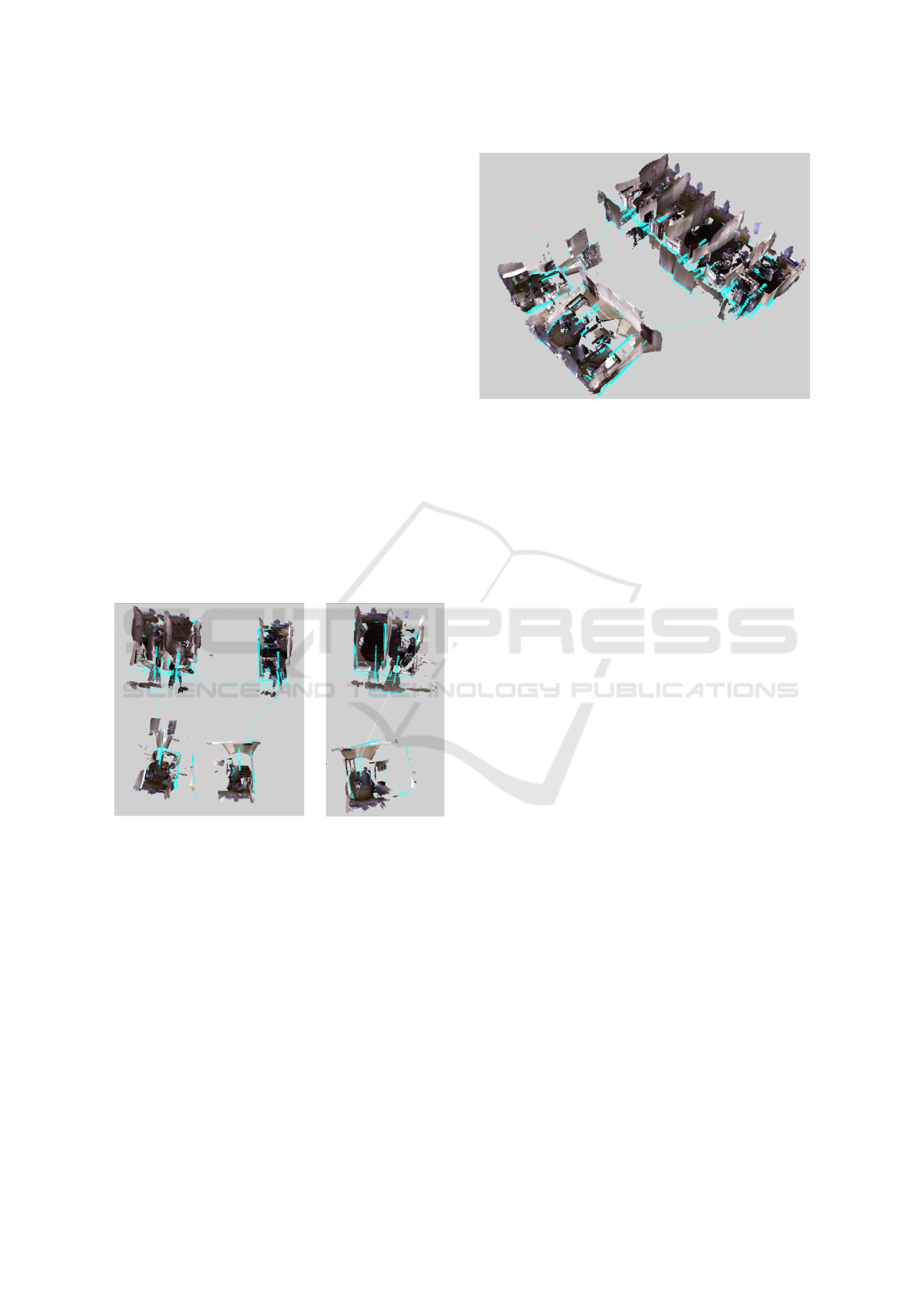
Finally, we show a 3D mapping of all rooms and
of the corridor in 11.
We also created some Rtabmap databases for each
action (movement and mapping) to show the possible
outcomes using simulated data. These are available at
http://tinyurl.com/zauoap8.
We found that both policies (with and without
groups) were really close in terms of the number of
steps necessary to perform the experiment and their
results. In both cases we reached a state where all
rooms were inspected (mapped). We noted a tendency
to try to perform unnecessary actions (like opening
an open door) while using groups. However, with
an higher level manager, those actions are checked
and only performed if consistent with the state of the
Figure 10: Merging of the mapping of both robots.
world, thus reducing the difference with the state of
the art solution.
8 CONCLUSION
In this paper, we solved a complex task, composed of
different complex or simple tasks, under uncertainty.
Our approach is based on the idea behind the H-
POMDP model and extends it to multiagent settings.
We defined a model allowing a problem formalized
by an MMDP to be split into smaller MMDPs, show-
ing that improvements can be achieved on the sub-
problems without a major loss in the solution quality.
We addressed the synchronization issue which is pre-
ponderant in a multiagent scenario and we described
experimental results obtained on a FSS problem. The
resolution of the Sub-MMDPs gave us insight into the
possible gain that can be achieved by reasoning on the
actions while solving complex problems. The drastic
cut in the transition numbers should allow us to tackle
a wider range of problems than with the current meth-
ods, while keeping a relatively good final policy. The
execution of the processed policies on a robotic plat-
form showed that even if the actions are sometimes
worse than in the optimal case, the agents are still per-
forming their task in the given amount of time step.
Future works will consist of solving such larger
problems, in terms of number of agents and environ-
ment, and adding a higher layer of decision to manage
the Sub-MMDPs in order to solve a problem using
different sets of sub-problems. The flexibility of the
presented model should allow us to add or remove ac-
tions during execution, which will give new methods
to manage open-MAS. We are working on an exten-
sion of this work to MPOMDP, Dec-MDP and Dec-
POMDP models with the management of belief states
during synchronization. We expect that by provid-
Dealing With Groups of Actions in Multiagent Markov Decision Processes
57

Figure 11: 3D Mapping of the rooms and corridor.
ing new tools based on this method, we will be able
to solve currently unmanageable complex multiagent
problems under uncertainty, and obtain good results.
REFERENCES
Becker, R., Zilberstein, S., Lesser, V., and Goldman, C. V.
(2004). Solving transition independent decentralized
Markov decision processes. Journal of Artificial Intel-
ligence Research, pages 423–455.
Bellman, R. (1954). The theory of dynamic programming.
Bull. Amer. Math. Soc. 60, no. 6, pages 503–515.
Bernstein, D. S., Zilberstein, S., and Immerman, N. (2000).
The complexity of decentralized control of markov
decision processes. In Proceedings of the Sixteenth
conference on Uncertainty in artificial intelligence,
pages 32–37. Morgan Kaufmann Publishers Inc.
Boutilier, C. (1996). Planning, learning and coordination in
multiagent decision processes. In Proceedings of the
6th conference on Theoretical aspects of rationality
and knowledge, pages 195–210. Morgan Kaufmann
Publishers Inc.
Boutilier, C. (1999). Sequential optimality and coordination
in multiagent systems. In IJCAI, volume 99, pages
478–485.
Claes, D., Robbel, P., Oliehoek, F. A., Tuyls, K., Hennes,
D., and van der Hoek, W. (2015). Effective approxi-
mations for multi-robot coordination in spatially dis-
tributed tasks. In Proceedings of the 2015 Interna-
tional Conference on Autonomous Agents and Multia-
gent Systems, AAMAS ’15, pages 881–890, Richland,
SC. International Foundation for Autonomous Agents
and Multiagent Systems.
Goldman, C. V. and Zilberstein, S. (2004). Decentral-
ized control of cooperative systems: Categorization
and complexity analysis. J. Artif. Intell. Res.(JAIR),
22:143–174.
Guestrin, C., Venkataraman, S., and Koller, D. (2002).
Context-specific multiagent coordination and plan-
ning with factored MDPs. In AAAI/IAAI, pages 253–
259.
Labbe, M. and Michaud, F. (2014). Online Global Loop
Closure Detection for Large-Scale Multi-Session
Graph-Based SLAM. In Proceedings of the IEEE/RSJ
International Conference on Intelligent Robots and
Systems, pages 2661–2666.
Littman, M., Dean, T., and Kaelbling, L. P. (1995). On the
complexity of solving markov decision problems. In
Uncertainty in Artificial Intelligence. Proceedings of
the 11th Conference, pages 394–402.
Matignon, L., Jeanpierre, L., and Mouaddib, A.-I. (2012).
Coordinated multi-robot exploration under communi-
cation constraints using decentralized markov deci-
sion processes. In AAAI, pages 2017–2023.
Melo, F. S. and Veloso, M. (2009). Learning of coordina-
tion: Exploiting sparse interactions in multiagent sys-
tems. In Proceedings of The 8th International Confer-
ence on Autonomous Agents and Multiagent Systems-
Volume 2, pages 773–780. International Foundation
for Autonomous Agents and Multiagent Systems.
Messias, J. V., Spaan, M. T., and Lima, P. U. (2013).
GSMDPs for Multi-Robot Sequential Decision-
Making. In AAAI.
Papadimitriou, C. H. and Tsitsiklis, J. N. (1987). The com-
plexity of markov decision processes. In Mathematics
of Operations Research 12(3), pages 441–450.
Parr, R. (1998). Flexible decomposition algorithms for
weakly coupled Markov decision problems. In Pro-
ceedings of the Fourteenth conference on Uncer-
tainty in artificial intelligence, pages 422–430. Mor-
gan Kaufmann Publishers Inc.
Pineau, J., Roy, N., and Thrun, S. (2001). A hierarchical ap-
proach to POMDP planning and execution. Workshop
on hierarchy and memory in reinforcement learning,
65(66):51–55.
Quigley, M., Conley, K., Gerkey, B. P., Faust, J., Foote, T.,
Leibs, J., Wheeler, R., and Ng, A. Y. (2009). Ros: an
open-source robot operating system. In ICRA Work-
shop on Open Source Software.
Witwicki, S. J. and Durfee, E. H. (2010). Influence-based
policy abstraction for weakly-coupled dec-POMDPs.
In ICAPS, pages 185–192.
Xuan, P., Lesser, V., and Zilberstein, S. (2001). Commu-
nication decisions in multi-agent cooperation: Model
and experiments. In Proceedings of the International
Joint Conference on Artificial Intelligence, pages
616–623.
ECTA 2016 - 8th International Conference on Evolutionary Computation Theory and Applications
58
