A Machine Learning Approach for Layout Inference in Spreadsheets

Elvis Koci

, Maik Thiele

, Oscar Romero

and Wolfgang Lehner

Database Technology Group, Department of Computer Science, Technische Universit

at Dresden, Dresden, Germany

Departament d’Enginyeria de Serveis i Sistemes d’Informaci

o (ESSI), Universitat Politecnica de Catalunya

(UPC-BarcelonaTech), C-Jordi Girona 1, Compus Nord, Barcelona, Spain

Keywords:

Speadsheets, Tabular, Layout, Structure, Machine Learning, Knowledge Discovery.

Abstract:

Spreadsheet applications are one of the most used tools for content generation and presentation in industry and

the Web. In spite of this success, there does not exist a comprehensive approach to automatically extract and

reuse the richness of data maintained in this format. The biggest obstacle is the lack of awareness about the

structure of the data in spreadsheets, which otherwise could provide the means to automatically understand

and extract knowledge from these ﬁles. In this paper, we propose a classiﬁcation approach to discover the

layout of tables in spreadsheets. Therefore, we focus on the cell level, considering a wide range of features not

covered before by related work. We evaluated the performance of our classiﬁers on a large dataset covering

three different corpora from various domains. Finally, our work includes a novel technique for detecting and

repairing incorrectly classiﬁed cells in a post-processing step. The experimental results show that our approach

delivers very high accuracy bringing us a crucial step closer towards automatic table extraction.

1 INTRODUCTION

Spreadsheet applications have evolved to be a tool

of great importance for transforming, analyzing, and

representing data in visual way. In industry, a consid-

erable amount of the company’s knowledge is stored

and managed in this form. Domain experts from these

companies use spreadsheets for ﬁnancial analysis, lo-

gistics and planning. Also, spreadsheets are a popular

format in the Web. Of particular importance are those

that can be found in Open Data platforms, where gov-

ernments, important institutions, and non proﬁt orga-

nizations are making their data available.

All this make spreadsheets a valuable source of

information. However, they are optimized to be user-

friendly rather than machine-friendly. The same data

can be formatted in different ways in a spreadsheet

depending on the information the user wants to con-

vey. It is relatively easy for humans to interpret the

presented information, but it is rather hard to do the

same algorithmically. As a result, we are constrained

to cumbersome approaches that limit the potential

reuses of data maintained in these types of ﬁles. A

typical problem that arises in most enterprises is that

due to the lack of visibility the data stored in spread-

sheets is not available for enterprise-wide data analy-

ses or reuse.

Our goal is to overcome these limitations by de-

veloping a method that allows to discover tables in

spreadsheets, infer their layout and other implicit in-

formation. We believe that this approach can provide

us with the means to extract a richer and more struc-

tured representation of data from spreadsheets. This

representation will act as the base for transforming the

data into other formats, such as a relational table or

a JSON document, depending on their characteristics

and the application requirements.

The relational model seems to be one of the nat-

ural progressions for spreadsheet data, since organiz-

ing data into a tabular layout is an essential aspect of

both worlds. By bringing spreadsheets and RDBMS

closer we can open the door to many applications.

For instance, it would be easier to digest them into

a data warehouse and perform complex data analy-

sis. Essentially, spreadsheets can become a substan-

tial source of data for existing or new business pro-

cesses.

In the literature, spreadsheet table detection has

only scarcely been investigated often assuming just

the same uniform table layout across all spreadsheets.

However, due to the manifold possibilities to struc-

ture tabular data within a spreadsheet, the assump-

tion of an uniform layout either excludes a substantial

number of tables and data from the extraction process

or leads to inaccurate results. Therefore, this paper

Koci, E., Thiele, M., Romero, O. and Lehner, W.

A Machine Lear ning Approach for Layout Inference in Spreadsheets.

DOI: 10.5220/0006052200770088

In Proceedings of the 8th International Joint Conference on Knowledge Discovery, Knowledge Engineering and Knowledge Management (IC3K 2016) - Volume 1: KDIR, pages 77-88

ISBN: 978-989-758-203-5

focuses on incorporating layout classiﬁcation in the

spreadsheet table extraction process. In detail, we ad-

dress the following aspects:

• Spreadsheet Building Blocks: Incorporating

lessons learned from spreadsheet research,

we propose ﬁve layout building blocks for

spreadsheet tables.

• Features: We consolidate and extend a wide

range of features proposed in the literature for

each of the building blocks. Using feature se-

lection, we evaluate the relevance of each feature

with respect to the classiﬁcation problem.

• Experimental Evaluation: We conduct an ex-

perimental evaluation on three spreadsheet cor-

pora and compare different classiﬁcation algo-

rithms.

• Handling Classiﬁcation Errors: We provide a

detailed discussion of classiﬁcation errors and

propose a novel technique to detect and repair

misclassiﬁed cells.

The paper is organized as follows: In Section 2 we

deﬁne the classiﬁcation problem for layout inference

in spreadsheets. The features used for the classiﬁca-

tion problem are listed in Section 3. In Section 4 we

describe how we annotated spreadsheets for the super-

vised learning. The results from the evaluation of the

proposed approach are summarized in Section 5. In

Section 6 we discuss how to handle misclassiﬁcation

in a post-processing task. Finally, we review related

work on table identiﬁcation and layout discovery in

Section 7.

2 THE CLASSIFICATION

PROBLEM

The objective of capturing the tabular data embedded

in spreadsheets can be treated as a classiﬁcation prob-

lem where the speciﬁc structures of a table have to

be identiﬁed. In the ﬁrst part of this section we de-

ﬁne these structures or building blocks that form our

classes. In the second part we specify the data item

granularity on which the classiﬁcation task will be

performed.

2.1 Spreadsheet Layout Building Blocks

Considering that tables embedded in spreadsheets

vary in shape and layout, it is required not only to

identify them but also recognize their building blocks.

We deﬁne ﬁve building blocks for spreadsheet tables:

Headers, Attributes, Metadata, Data and Derived (see

Figure 1: The Building Blocks.

Figure 1). A “Header” (H) cell represents the label

of a column and can be ﬂat or hierarchical (stacked).

Hierarchical structures can be also found in the left-

most or right-most columns of a table, which we call

“Attributes” (A), a term ﬁrst introduced in (Chen and

Cafarella, 2013). Attributes can be seen as instances

from the same or different (relational) dimensions

placed in one or multiple columns in a way that con-

veys the existence of a hierarchy. We label cells as

“Metadata” (M) when they provide additional infor-

mation about the table as a whole or its speciﬁc sec-

tions. Examples of Metadata are the table name, cre-

ation date, and the unit for the values of a column. The

remaining cells form the actual payload of the table

and are labeled as “Data”. Additionally, we use the

label “Derived” (B) to distinguish those cells that are

aggregations of other Data cells’ values. Derived cells

can have a different structure from the core Data cells,

therefore we need to treat them separately. Figure 1

provides examples of all the aforementioned building

blocks.

2.2 Working at the Cell Granularity

One potential solution for the table identiﬁcation and

layout recognition tasks would be to operate un-

der some assumptions about the typical structure of

spreadsheet tables. That means expecting spread-

sheets to contain one or more tables with typical lay-

outs that are well separated from each other. In such

scenario we could deﬁne simple rules and heuristics

to recognize the different parts. For example, the

top row could be marked as Header when it contains

mostly string values. Additionally, cells containing

the string “Table:” are most probably Metadata. How-

ever, this approach can not scale to handle arbitrary

spreadsheet tables. Since, the corpora we have con-

sidered include spreadsheets from various domains,

we need to ﬁnd a more accurate and more general so-

lution.

For this reason, our approach focuses on the

KDIR 2016 - 8th International Conference on Knowledge Discovery and Information Retrieval

Figure 2: The Cell Classiﬁcation Process.

smallest structural unit of a spreadsheet, namely the

cell. At this granularity we are able to identify ar-

bitrary layout structures, which might be neglected

otherwise. For instance, it is tricky to classify rows

when multiple tables are stacked horizontally. The

same applies for the cases when Metadata are inter-

mingled with Header or Data. Nevertheless, we ac-

knowledge that the probability of having misclassiﬁ-

cations increases when working with cells instead of

composite structures such as rows or columns. There-

fore, our aim is to come up with novel solutions that

mitigate this drawback.

Figure 2 illustrates the three high-level tasks that

compose our cell classiﬁcation process. Initially, the

application reads the spreadsheet ﬁle and extracts the

features of each non-blank cell. Here we considered

different aspects of the cell, summarized in Section 3.

In the next step, cells are classiﬁed with very high

accuracy (see Section 5.2) based on their features. Fi-

nally, a post-processing step improves the accuracy

of the classiﬁer even further by applying a set of rules

that are able to identify cells that are most probably

misclassiﬁed and have to be relabeled.

To complete the picture, Figure 2 also includes

the Table Reconstruction task, which forms a separate

topic and is therefore left as future work.

3 FEATURE SPECIFICATION

In this paper we consider cell features especially for

Microsoft Excel spreadsheets. However, most of

the features listed in the next sections can be used

for other spreadsheet tools as well. To process the

spreadsheet ﬁles and extract the features we are using

Apache POI

, which is the most complete Java library

for handling Excel documents. Many of the features

listed below are directly accessible via the classes of

this library. Others require a custom implementation.

More details on this project can be found on our web-

site

. These features incorporate and extend the fea-

tures proposed by (Adelﬁo and Samet, 2013; Chen

https://poi.apache.org/

https://wwwdb.inf.tu-dresden.de/misc/DeExcelarator

and Cafarella, 2013; Eberius et al., 2015)

3.1 Content Features

The content features describe the cell value, but not

its format. We have considered the cell type (numeric,

string, boolean, date, or formula), and whether the cell

is a hyperlink or not. For numeric cells we check if

the value is within a speciﬁed year range, to distin-

guish values that could also be interpreted as dates.

Furthermore, we record the length of the value and

the number of tokens that compose it. The latter is

always one for non-string cells. Finally, we have de-

ﬁned 13 textual features relevant only to cells con-

taining string values. We have listed below a subset

of these features.

• IS CAPITALIZED: Whether the string is in title

case.

• STARTS WITH SPECIAL: True, if the ﬁrst character

is a special symbol.

• IS ALPHANUMERIC: Whether the string contains

only alphabetic and numeric characters.

• CONTAINS PUNCTUATIONS : True, if the string

contains punctuation characters. Here, we are not

considering the colon character, which is the sub-

ject of separate feature.

• WORDS LIKE TOTAL: If the string contains tokens

like “total”, “sum”, and “max”, this feature is set

to true.

3.2 Cell Style Features

In addition to content features, the style of the cell

can provide valuable indicators for the classiﬁcation

process. Since the total number of these features is

large, we have arranged them below into subgroups.

• ALIGNMENT: Type of horizontal and vertical align-

ment, and number of indentations.

• FILL: Whether the cell is ﬁlled with a color or not,

and the type of ﬁll pattern.

• ORIENTATION: Whether the contents are rotated.

A Machine Learning Approach for Layout Inference in Spreadsheets

• CONTROL: Checks if the options “wrap text” and

“shrink to ﬁt” are set to true.

• MERGE: Checks if the cell is merged and record

the number of cells in the merged region. If not

merged, it is set to 1.

• BORDERS: The type of the top, bottom, left, and

right border. Excel supports 14 border types.

Also, we count the number (from 0 to 4) of de-

ﬁned borders for the cell.

3.3 Font Features

The features of this group describe the font of the cell.

We have considered various aspects of the font, such

as its size, effects, style and color.

• FONT COLOR DEFAULT: Whether the font color is

the default one (i.e., black) or not.

• FONT SIZE: A numeric value between 1 and 409.

• IS BOLD: Whether the font is bold.

• IS ITALIC: Whether the font is italic.

• IS STRIKE OUT: Whether the font is striked out.

• UNDERLINE TYPE: Single, single accounting, dou-

ble, double accounting, none.

• OFFSET TYPE: Superscript, subscript or none.

• FORMATTING RUNS: Number of unique formats in

the cell.

3.4 Reference Features

These features explore the Excel formulas and their

references in the same or other worksheets. Here, not

only have we considered references from the same

worksheet (intra-references), but also references from

the other worksheets in the ﬁle (inter-references). The

observation is that the formula cells are mostly found

in Data or Derived regions, and that the cells refer-

enced by these formulas are predominantly Data. Be-

low, we list the features used in our analysis.

• FORMULA VAL TYPE: The result of the formula can

be numeric, string, boolean, date, or not applica-

ble (n/a).

• IS AGGREGATION FORMULA: Whether the formula

is an aggregation or not.

• REF VAL TYPE: The referencing formula can out-

put a numeric, string, boolean, date, or not appli-

cable (n/a).

• REF IS AGGREGATION FORMULA: Whether the ref-

erencing formula is an aggregation or not.

We had to introduce the value “Not Applicable” for

each of these features, since there are cells that do not

contain formulas and are not referenced by a formula.

3.5 Spatial Features

We have also considered features that describe the

“neighborhood” of the cell. This includes the location

of the cells (deﬁned by the row and column number)

and the features of its neighbors. Only the neighbors

that share a border (edge) with the cell are inspected,

i.e., the top, down, left, and right. When the neigh-

boring cells are blank or outside of the bounds of the

sheet, we set the value of the corresponding features

to “Not Applicable” (n/a).

• ROW NUM: The index of the row the cell is located

in.

• COLUMN NUM: The index of the column the cell is

located in.

• NUMBER OF NEIGHBORS: The number (from 0 to

4) of neighboring cells that are not blank. For

merged cells, we consider each side (the top and

bottom row, and the left and right column) in an

aggregated manner. If there is at least one non-

blank cell, the side is considered as active and thus

marked as 1. Otherwise, we mark it as 0.

• MATCHES {TOP,BOTTOM,LEFT,RIGHT} STYLE:

Whether the neighbor has the same style as the

cell.

• MATCHES {TOP,BOTTOM,LEFT,RIGHT} TYPE:

Whether the neighbor has the same content type

as the cell.

• {TOP,BOTTOM,LEFT,RIGHT} NEIGHBOR TYPE:

The content type of the neighbor. It can take one

of the values mentioned in Section 3.1.

4 CREATING THE GROUND

TRUTH

The supervised classiﬁcation processes requires a

ground truth dataset, which is used for both training

and validation. In Section 4.1 we brieﬂy describe the

three spreadsheet corpora used to extract and gener-

ate a representative set of spreadsheets. To create the

training data we developed a spreadsheet labeling tool

(see Section 4.2) that provides the means to annotate

ranges of cells. Given that tool, we randomly selected

and annotated ﬁles from the three corpora for which

we provide statistics in Section 4.3.

4.1 Spreadsheet Corpora and Training

Data

For our experiments we have considered spreadsheets

from three different sources. Euses (Fisher and

KDIR 2016 - 8th International Conference on Knowledge Discovery and Information Retrieval

Rothermel, 2005) is one of the oldest and most

frequently used corpora. It has 4, 498 unique spread-

sheets, which are gathered through Google searches

using keywords such as “ﬁnancial” and “inventory”.

The Enron corpus (Hermans and Murphy-Hill, 2015)

contains over 15, 000 spreadsheets, extracted from the

Enron email archive. This corpus is of particular in-

terest, since it provides access to real-world business

spreadsheets used in industry. The third corpus is

Fuse (Barik et al., 2015) that contains 249, 376 unique

spreadsheets, extracted from Common Crawl

. Each

spreadsheet in Fuse is accompanied by a JSON ﬁle

that contains metadata and statistics. Unlike the other

two corpora, Fuse can be reproduced and extended.

4.2 The Annotation Tool

Using the Eclipse SWT

library we developed an in-

teractive desktop application that ensures good qual-

ity annotations. The original Excel spreadsheet is em-

bedded into a Java window and protected from user

alteration. To create an annotation, the user selects

a range of cells (region) and then chooses the appro-

priate predeﬁned label. A rectangle, which is ﬁlled

with the color associated to the label, covers the an-

notated region. The application evaluates the anno-

tations and rejects the inappropriate ones. For exam-

ple, the user cannot annotate ranges that are empty or

overlapping with existing annotations. The data from

all the created annotations are stored in a new sheet,

named “Range Annotation Data”. This sheet is pro-

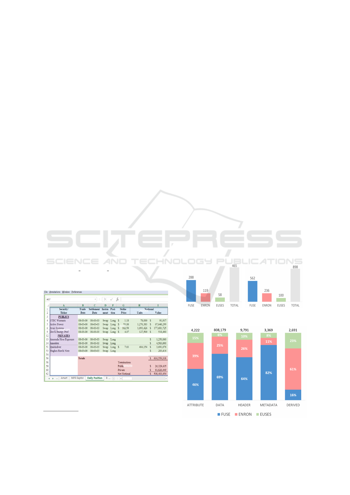
tected and hidden once the ﬁle is closed. Figure 3

provides an example of an annotated sheet.

Figure 3: Annotated Sheet.

In addition to the building block described in Sec-

tion 2, we have introduced the possibility to annotate

http://commoncrawl.org/

https://www.eclipse.org/swt/

a region (area) that represents a whole table. A rect-

angle with thick blue borders marks its boundaries.

We need the “Table” annotation for two main reasons:

Firstly, we can govern the labeling process, to assure

valid annotations. For example, Data can only exist

inside a Table. However, Metadata can be left out-

side when they provide information relevant to mul-

tiple Tables. Secondly, these annotations will help us

evaluate the Table Reconstruction task, in the future.

4.3 Annotation Statistics

The graphs below provide an overview of the col-

lected annotations and the contribution of each cor-

pus.

We considered each corpus individually and as-

signed a unique number to their ﬁles. Using a random

number generator we extracted subsets of ﬁles. From

these, we annotated a total of 465 worksheets (216

ﬁles) and 898 tables.

In Figure 5 we examine the annotated cells. The

total number of cells for each label (class) is placed at

the top of the column bar. There was a small amount

of cells that did not match any of the deﬁned labels.

These are usually random notes that do not have a

clear function and do not provide additional context

(information) about the table. We decided to omit

such cells.

As can be seen in Figure 5, the number of Data

cells is by orders of magnitude larger than the other

(a) Sheets (b) Tables

Figure 4: Annotation Statistics.

Figure 5: Annotated Cells.

A Machine Learning Approach for Layout Inference in Spreadsheets

label numbers. To adjust the class distribution we un-

dersampled the Data class, considering only the most

difﬁcult case, which are the ﬁrst and the last row and

three random rows in between. By applying this tech-

nique the Data class was reduced to 32, 875 instead of

808, 179 cells. Considering also the other four classes

the ﬁnal gold standard consists of 52, 948 cells in to-

tal.

Also, Figure 5 provides a look into the character-

istics of the three corpora. For instance, the selected

spreadsheets from Enron corpus are more likely to

contain Derived cells (aggregations). This result is

somehow expected since, as stated before, Enron

spreadsheets are coming from the industry, which is

characterized by a heavier use of formulas. Also, Eu-

ses has a high contribution in the Derived cells con-

sidering the number of annotated sheets from this cor-

pus. Moreover, we observe that Fuse contributes the

vast majority of Metadata cells. Enron and Euses have

a high contribution in the Attribute cells. These char-

acteristics surely inﬂuence the classiﬁcation results,

which are discussed in Section 5.

5 EVALUATION

5.1 Feature Selection

We used Weka

, a well known tool for machine learn-

ing tasks, for feature selection and classiﬁcation. Ini-

tially, we binarized nominal features with more than

two values, which gave us 219 features in total. We

used the “RemoveUseless” option to remove the fea-

tures that do not vary at all or vary too much. Addi-

tionally, we manually removed those features that are

practically constant (i.e., at least 99.9% of cases the

value is the same). Furthermore, we decided to ex-

clude from the ﬁnal set features that check the style

and content type of the neighbors (see last 3 items in

Section 3.5). These features will be subject of future

experiments related both to the classiﬁcation task and

the post-processing step. We provide more details on

this matter in Section 6.

The remaining 88 features were evaluated

using the InfoGainAttribute, GainRatioAttribute,

ChiSquaredAttribute, ConsitencySubset, and CfsSub-

set feature selection methods. For each one of them

we performed 10 folds (runs). A bidirectional Best

First search was used for ConsitencySubset and Cfs-

Subset, while the other methods can only be coupled

with Ranker search.

http://www.cs.waikato.ac.nz/ml/weka/

From the results we considered most of the fea-

tures that score high in these selection methods. Al-

though, we were predominantly inﬂuenced by Con-

sistencySubset results, since ,when tested, they pro-

vide the highest classiﬁcation accuracy for the small-

est number of features. We also included in the ﬁ-

nal set features that are strong indicators despite the

fact that they describe small number of instances.

“Words Like Table” is an example of such features,

where 48 out of total 49 positive (true) cases are in-

stances of the Metadata class.

Table 1: Selected Content and Style Features.

Content Cell Style

LENGTH# IDENTATIONS#

NUM OF TOKENS# H ALIGNMENT DEFAULT?

LEADING SPACES# H ALIGNMENT CENTER?

IS NUMERIC? V ALIGNMENT BOTTOM?

IS FORMULA? FILL PATTERN DEFAULT?

STARTS WITH NUMBER? IS WRAPTEXT?

STARTS WITH SPECIAL? NUM OF CELLS#

IS CAPITALIZED? NONE TOP BORDER?

IS UPPER CASE? THIN TOP BORDER?

IS ALPHABETIC? NONE BOTTOM BORDER?

CONTAINS SPECIAL CHARS? NONE LEFT BORDER?

CONTAINS PUNCTUATIONS? NONE RIGHT BORDER?

CONTAINS COLON? MEDIUM RIGHT BORDER?

WORDS LIKE TOTAL? HAS 0 DEFINED BORDERS?

WORDS LIKE TABLE?

IN YEAR RANGE?

Table 2: Selected Font, Reference and Spatial Features.

Font Reference Spatial

FONT SIZE# IS AGGRE FORMULA? ROW NUMBER#

FONT COLOR DEFAULT? REF VAL NUMERIC? COL NUMBER#

IS BOLD? HAS 0 NEIGHBORS?

NONE UNDERLINE? HAS 1 NEIGHBOR?

HAS 2 NEIGHBORS?

HAS 3 NEIGHBORS?

HAS 4 NEIGHBORS?

Table 1 and 2 list the selected features, 43 in to-

tal. Those sufﬁxed with ? represent boolean features.

While, those sufﬁxed with # represent numeric fea-

tures.

The results from the classiﬁcation evaluation, de-

scribed in Section 5.2, show that the above features

are good indicators for the ground truth dataset. How-

ever, in general spreadsheets exhibit different charac-

teristics depending on the domain they come from.

For example, we expect that reference features are

more important for industrial rather than for Web

spreadsheets, since the former are characterized by

heavier use of formulas. Therefore, an independent

feature selection might be required for other spread-

sheet datasets in order to achieve near optimum accu-

racy. Nevertheless, in the appendix we provide more

details about the feature selection results from our ex-

periments.

KDIR 2016 - 8th International Conference on Knowledge Discovery and Information Retrieval

5.2 Classiﬁers

In our evaluation, we consider various classiﬁcation

algorithms, most of which have been successfully

applied to similar tasks in the literature. Speciﬁcally,

we consider CART (Breiman et al., 1984) (Simple-

CART in Weka), C4.5 (Quinlan, 1993) (J48 in Weka),

Random Forest (Breiman, 2001) and support vector

machines (Vapnik, 1982) (SMO in Weka), which

uses the sequential minimal optimization algorithm

developed by (Platt, 1998) to train the classiﬁer. Here

we consider both a polynomial kernel and an RBF

kernel. We evaluate the classiﬁcation performance

using 10-fold cross validation. The results of our

evaluation are displayed in Table 3.

Table 3: Classiﬁer Evaluation: All measures are reported as

percentages for the following classes: Attribute (A), Data

(D), Header (H), Metadata (M), and Derived (B).

Classiﬁer Metric A D H M B Weight. Avg.

Rand. Forest Precision 96.9 98.6 97.9 97.8 97.7 98.2

Recall 96.8 99.2 98.0 94.1 94.2 98.2

F1 96.8 98.9 98.0 95.9 95.9 98.2

J48 Precision 95.1 98.1 95.9 93.9 96.4 97.1

Recall 94.8 98.5 96.1 92.1 93.6 97.1

F1 94.9 98.3 96.0 93.0 95.0 97.1

Simple Cart Precision 94.3 97.6 95.1 92.1 95.2 96.4

Recall 94.3 98.0 95.3 89.8 92.2 96.4

F1 94.3 97.8 95.2 91.0 93.7 96.4

SMO Poly Precision 89.7 95.1 93.7 89.8 93.6 94.0

Recall 94.7 96.9 90.1 83.1 84.9 94.0

F1 92.2 96.0 91.9 86.3 89.1 94.0

SMO Rbf Precision 88.6 93.7 91.6 91.9 94.9 92.8

Recall 91.9 97.4 89.0 70.3 80.9 92.8

F1 90.2 95.5 90.3 79.6 87.3 92.7

As can be seen in this table, the scores for all the

classes (labels) are satisfactory. We note that deci-

sion tree based classiﬁers perform better than SMO in

this classiﬁcation task. In particular, Random Forest

produces the highest results. Another interesting fact

is that all the classiﬁers perform worst with Metadata

and Derived classes. The main reason, seems to be

low recall for these classes.

Table 4: Random Forest Confusion Matrix.

Total A D H M B

4222 4087 88 29 18 0 Attributes

32875 70 32626 86 33 60 Data

9791 36 139 9597 19 0 Header

3369 26 86 88 3169 0 Metadata

2691 0 153 2 0 2536 Derived

Table 4 displays the confusion matrix from the

evaluation of the Random Forest classiﬁer. The values

with bold font, in the diagonal of the matrix, represent

the number of correctly classiﬁed cells per label. We

have marked with red color the “problematic” values.

There is a considerable number of incorrectly clas-

siﬁed data cells, as can be seen in the second row.

However, the bigger concern is that other classes are

often misclassiﬁed as data (see second column). This

was somehow expected for Derived cells, since they

are close (similar) to the Data cells. These misclas-

siﬁcations together with the low number of instances

are the main reasons for the low recall of the Derived

class. Also, we note that Metadata cells tend to be

falsely classiﬁed as Header and Data, which conse-

quently impacts the recall of this class. One poten-

tial reason for these results can be the big variety of

Metadata cells. In other words, these cells do not ex-

hibit the level of homogeneity found in other classes

of cells.

To provide a more concrete picture on the accu-

racy of the classiﬁcation, we decided to train and run

10-fold cross validation using Random Forest classi-

ﬁer on the full dataset of annotated cells (828, 252)

with the selected features. The F1 measure does not

change much for the Attributes (96.6%) and Header

(97.7%) cells. The classiﬁer scores 99.9% on F1 mea-

sure for Data cells, since the full dataset contains a

vast number of instances of this class. The F1 mea-

sure decreases for Metadata and Derived, 93.5% and

94.9% respectively.

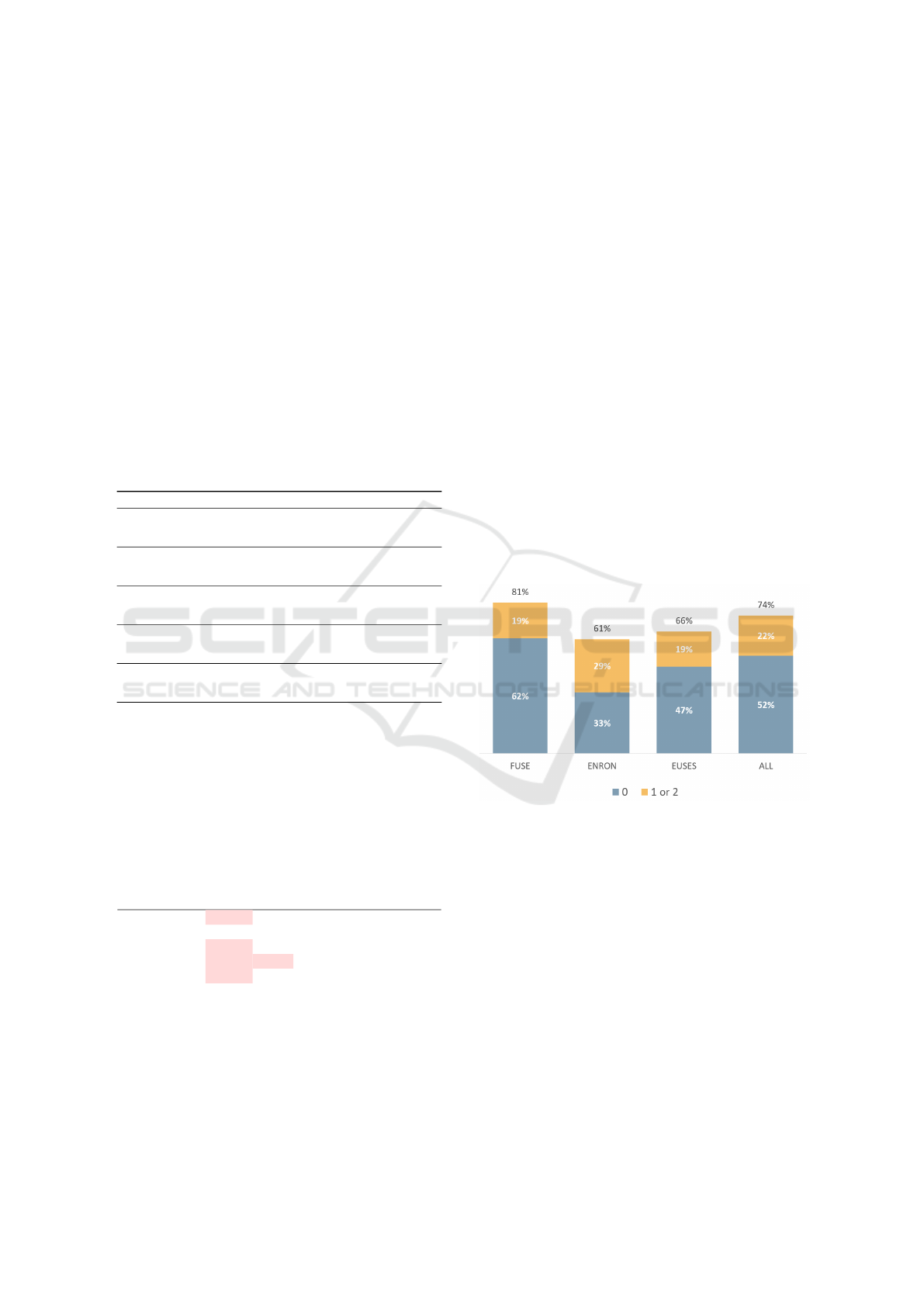
Figure 6: Percentage of Sheets with 2 or Less Misclassiﬁ-

cations.

Figure 6 displays the percentage of sheets for

which the classiﬁer has misclassiﬁed 2 or less cells.

We have stacked those cases that have 0 misclassiﬁ-

cation with those that have 1 or 2. We observe that

more than half of the sheets are classiﬁed with no er-

rors. Also, we notice that the classiﬁer has the highest

accuracy in the Fuse sheets and the lowest in the En-

ron sheets.

6 POST-PROCESSING

The objective of the post-processing phase (Step 3

in Figure 2) is to detect and repair misclassiﬁcations

based on spatial patterns (rules) which were deduced

A Machine Learning Approach for Layout Inference in Spreadsheets

from an empirical study of the classiﬁcation results.

We believe that unusual arrangements of labels could

hint the existence of misclassiﬁcations. For exam-

ple, ﬁnding a Data cell in a row that otherwise has

only Header cells is considered to be unexpected. The

same can be said when an Attribute cell is completely

surrounded by instances of the Metadata class.

Identifying incorrectly classiﬁed cells is only one

part of the repairing process. We would also like to

update the labels of these cells. Again here we con-

sider the arrangement of labels close to the cell, which

we will refer to as the neighborhood of the cell. In the

examples provided above, inﬂuenced by the neighbor-

hood, we would have updated the labels to Header and

Metadata respectively.

As seen from the examples, the classiﬁcation la-

bels provide a valuable context. Since our evaluation

shows that the classiﬁcation process has high accu-

racy, we expect the vast majority of identiﬁed cases

to be true positives. In other words, we assume that

the neighborhood of the cell mostly contains correctly

classiﬁed cells. In the following sections we discuss

in more detail the identiﬁcation and relabeling steps.

6.1 Misclassiﬁcation Patterns

We studied misclassiﬁcation patterns in the classiﬁ-

cation results for the full dataset of annotated cells.

From 1, 237 misclassiﬁed cells, we identiﬁed 672

unique patterns. From the ﬁrst 40 most repeated pat-

terns we inferred generic (for all labels) rules to dis-

cover misclassiﬁcations. Below we discuss ﬁve of

these rules.

Here our intention is to provide the intuition be-

hind each rule (pattern), rather than its speciﬁc im-

plementation. Figure 7 provides a visual represen-

tation of the considered rules. The cells ﬁlled with

green lines (Inﬂuencer) represent neighbors that share

the same label but different from the one ﬁlled with

red dots (i.e., the potential misclassiﬁcation). The

“Tunel” pattern tries to identify cells that are com-

pletely or partially surrounded by instances of a dif-

ferent cell class. We only consider the instances of

these pattern that occur horizontally.

In Figure 7.a we display one of the two possible

arrangements of this pattern. The “T-block” pattern

identiﬁes misclassiﬁcations that occur in the border

between two different sections of the table. In addi-

tion to the one presented in Figure 7.b, the T-block

pattern can also occur when the “head” of the T-shape

is on the top row. The “Attribute Interrupter” (AIN)

pattern applies to Attribute cells (see Figure 7.c). For

this reason, AIN has a vertical nature. The intention

is to identify misclassiﬁed cells in Attribute columns.

(a) Tunel (b) T-blocks (c) AIN

(d) RIN (e) Corner

Figure 7: Misclassiﬁcation Patterns.

The “Row Interrupter” (RIN) pattern discovers the

cases when a row is “invaded” by a cell of another

class. Figure 7.d displays the arrangement for this

pattern. Finally, the “Corner” pattern discovers mis-

classiﬁcations that occur in the corners of the table.

Therefore, there are four possible versions of this pat-

tern. Figure 7.e displays one of them. In this ﬁgure

we do not display the cells on the left and bottom,

since they are supposed to be blank or undeﬁned (i.e.,

outside of the sheet borders).

Table 5 displays the number of times each pat-

tern occurs in the classiﬁcation results. We should

note that the patterns are not mutually exclusive. In

the majority of times these patterns match incorrectly

classiﬁed cells. However, we also have a considerable

number of cases that the cell was correctly classiﬁed.

Table 5: Pattern Occurrences.

Pattern

Incorrectly

Classiﬁed

Correctly

Classiﬁed

Total

Tunel 45 12 57

AIN 41 1 42

RIN 29 4 33

T-blocks 28 1 29

Corner 13 2 15

6.2 Relabeling

In this section we describe our strategy for relabeling

the misclassiﬁed cells based on the matched pattern.

Essentially, we infer the new label from the neighbor-

ing cells we call “Inﬂuencers” (see Figure 7). For the

Tunel pattern we update the label to match the ma-

jority of the close-neighbors. When the T-block pat-

tern is identiﬁed, the label of the right and left close-

neighbors is used. We set the label for the central cell

to Attribute, when the AIN pattern occurs. For the

RIN pattern we ﬂip the label to match the rest of the

KDIR 2016 - 8th International Conference on Knowledge Discovery and Information Retrieval

row. Finally, when the Corner pattern occurs, the la-

bel of the cell is updated to the match the rest of the

neighbors.

We decided to evaluate our approach, this time

ﬂipping the label of the identiﬁed cells. We performed

these updates using all the patterns in a sequential

run. The updated list of labels from the occurrences

of the previous pattern becomes the input for the next

pattern. To avoid overlaps between them, we allow

updating the cell label only once. The patterns were

used in the ascending order of the number of correctly

classiﬁed cells they matched (see Table 5): AIN, T-

Blocks, Corner, RIN, Tunel. The results show that

we managed to repair 152 misclassiﬁed and lose 14

correctly classiﬁed. Table 6 summarizes the results of

this execution per label. Also, in Table 7 we provide

the updated F1 measures after the relabeling for the

full dataset of cells.

Table 6: Label Flips.

Attributes Data Header Metadata Derived

Gained

41 57 26 18 10

Lost

0 1 8 3 2

Table 7: F1 measures before and after relabeling.

Attributes Data Header Metadata Derived

Original

96.6 99.9 97.7 93.5 94.9

Relabeled

97.3 99.9 97.9 94 95.2

There is potential in using patterns for handling

misclassiﬁcations in a post-processing step. However,

this approach needs further reﬁnement. We believe

that one way to improve it is by taking in consid-

eration the type and style of the neighbors. During

the classiﬁcation process these features provide a mi-

nor improvement. However, under the label context

they should be able to provide us with stronger indica-

tions. We are also looking at methods for discovering

patterns automatically. The main aim is to identify

patterns that apply to speciﬁc classes, since we ex-

pect them to be more accurate than the generic ones.

The results displayed in Table 6 hint towards this di-

rection. Finally, we need to avoid overﬁtting on the

current classiﬁcation results. Hence, we plan in the

future to perform tests in multiple samples.

7 RELATED WORK

7.1 Spreadsheet Layout Inference

The paper (Chen and Cafarella, 2013) describes

work on automatic extraction of relational data from

spreadsheets. The proposed approach processes

data frame spreadsheets (i.e., containing attributes or

metadata regions on the top/left and a block of nu-

meric values). In particular, the authors focus their

efforts on hierarchical spreadsheets (i.e., hierarchical

left or top attribute regions). They have used machine

learning techniques and few heuristics (i) to identify

the regions (layout) of the data frames and (ii) to ex-

tract the hierarchy of the attributes. This then be-

comes the input for the (iii) extraction of data in the

form of relational tuples. The extension of this work

is reported in (Chen and Cafarella, 2014). From the

ﬁrst paper, we isolate the structure discovery meth-

ods, which are closely related to our research prob-

lem. In contrast to us, their approach is to classify

the rows in a spreadsheet using linear-chain, condi-

tional random ﬁeld (CRF). Their evaluation is per-

formed on 100 random hierarchical spreadsheets from

their corpus (called Web). The results show that their

method, similar to us, has high accuracy for regions

that contain Data. However, for the remaining labels

the scores are lower. We should note that they have

not deﬁned a separate class for Derived cells. Also,

what we call “Metadata” is further distinguished into

two separate classes, “Title” and “Footer”. In ad-

dition to this, the authors have established a set of

assumptions for the arrangement of data in spread-

sheets. Cases that do not comply to these expecta-

tions are simply not treated by their system. However,

as we argue in Section 2, the classiﬁcation at the row

level together with the assumptions about the struc-

ture limit the abilities of the system.

Work on the extraction of schema from Web tab-

ular data, including spreadsheets, is presented in

(Adelﬁo and Samet, 2013). The authors have tested

various approaches to identify the layout of the ta-

bles in spreadsheets. All of them work on the row

level. Their evaluation shows that the most promising

results are achieved when a CRF classiﬁer is used to-

gether with their novel approach for encoding cell fea-

tures into row features (called “logarithmic binning”).

In contrast to us, they have considered a much smaller

number of cell features (15 in total), since their ap-

proach had to work for both spreadsheets and HTML

tables. There are some differences with what regards

the deﬁned labels. They have further differentiated

between simple and stacked Headers. Also, they have

not deﬁned a separate label for Attributes cells. More-

over, they have deﬁned two kinds of Metadata: “Title”

and “Non-relational”. Another aspect that differenti-

ates our work from theirs, is that we have considered

in our analysis industrial spreadsheets in addition to

the ones collected from the Web.

In (Eberius et al., 2013), the authors present De-

Excelerator, a framework which takes as input par-

A Machine Learning Approach for Layout Inference in Spreadsheets

tially structured documents, including spreadsheets,

and automatically transforms them into ﬁrst normal

form relations. Their approach works based on a

set of rules and heuristics. For spreadsheets, these

have resulted from a manual study on real-world ex-

amples. The performance of the framework was as-

sessed by a group of 10 database students, on sample

of 50 spreadsheets extracted from data.gov. DeExcel-

erator received good scores for all the various tasks

it handles, including layout inference. Nevertheless,

we believe that our approach is much more powerful,

since the best features are learned automatically from

the annotated spreadsheets. Moreover, we have per-

formed our evaluation on a considerably larger sam-

ple, consisting of spreadsheets from various domains

and sources.

Techniques for header and unit inference for

spreadsheets are discussed in (Abraham and Erwig,

2004). This paper looks in the same research prob-

lem as us from a software engineering perspective.

The core idea is that formula (reference) errors can

be discovered more accurately in spreadsheets once

the system is aware of the table structure. To achieve

this, they have developed several spatial algorithms

(strategies), and a weighting scheme that combines

their results. Same as us, they work on the cell level,

but they use heuristics instead of learning methods.

They have deﬁned four possible semantical labels for

a cell. The notion of Metadata cells does not exist in

their analysis. For the other classes we can ﬁnd sim-

ilarities with the ones we have deﬁned. They have

performed their evaluation on two datasets, consist-

ing of 10 and 18 spreadsheets correspondingly. The

results from their evaluation are encouraging. How-

ever, the lack of reproducibility and the small size of

these datasets makes it difﬁcult to judge this approach

in much more general context.

7.2 Table Recognition and Layout

Discovery

One of the typical ways to present information (facts)

is by organizing data in a tabular format. As a result,

the problems of table recognition and layout discov-

ery have been encountered by various research com-

munities. Some of the most recent studies are related

to HTML (Web) tables. In (Wang and Hu, 2002), de-

cision trees and support vector machines (SVM) are

considered to differentiate between genuine and non-

genuine Web tables. The authors deﬁned structural,

content type, and a word group features. The (Crestan

and Pantel, 2011) reports the study of large sample of

Web tables, which yielded a taxonomy of table lay-

outs. It also discusses heuristics, which are based on

features similar to the paper above, to classify Web

tables into the proposed taxonomy. In (Eberius et al.,

2015), the authors describe the creation of the Dres-

den Web Table Corpus, by proposing a classiﬁcation

approach that works on the level of different table lay-

out classes.

8 CONCLUSIONS

In conclusion, we have presented our approach for

discovering the layout (structure) of the data in

spreadsheets. The ﬁrst aspect of this approach in-

volves classifying the individual non-blank cells. Us-

ing our specialized tool, we have labeled the cells

from a considerable number of sheets, taken from var-

ious domains. The experiments show that our models

have high accuracy and perform well with all the de-

ﬁned classes. The best results are achieved when Ran-

dom Forest is used to build the classiﬁcation model.

Moreover, in this paper we discuss a technique for

identifying and correcting misclassiﬁcations. The cell

and its neighbors (i.e., cells adjacent to it) are ana-

lyzed for improbable label arrangements (patterns).

We update the label of the potentially misclassiﬁed

cell based on the matched pattern. Although not yet

mature, the results from the evaluation of this method

are encouraging. It is our aim, in the future, to work

on more elaborate techniques for identifying patterns

pointing to incorrectly classiﬁed cells. Also, part of

our future plans is to work on the identiﬁcation of the

individual tables in a spreadsheet from the ﬁnal output

of our classiﬁcation approach.

ACKNOWLEDGEMENTS

This research has been funded by the European Com-

mission through the Erasmus Mundus Joint Doctorate

“Information Technologies for Business Intelligence -

Doctoral College” (IT4BI-DC).

REFERENCES

Abraham, R. and Erwig, M. (2004). Header and unit in-

ference for spreadsheets through spatial analyses. In

VL/HCC’04, pages 165–172. IEEE.

Adelﬁo, M. D. and Samet, H. (2013). Schema extraction

for tabular data on the web. VLDB’13, 6(6):421–432.

Barik, T., Lubick, K., Smith, J., Slankas, J., and Murphy-

Hill, E. (2015). FUSE: A Reproducible, Extendable,

Internet-scale Corpus of Spreadsheets. In MSR’15.

KDIR 2016 - 8th International Conference on Knowledge Discovery and Information Retrieval

Breiman, L. (2001). Random forests. Machine Learning,

45(1):5–32.

Breiman, L., Friedman, J., Olshen, R., and Stone, C. (1984).

Classiﬁcation and Regression Trees. Wadsworth.

Chen, Z. and Cafarella, M. (2013). Automatic web spread-

sheet data extraction. In SSW’13, page 1. ACM.

Chen, Z. and Cafarella, M. (2014). Integrating spread-

sheet data via accurate and low-effort extraction. In

SIGKDD’14, pages 1126–1135. ACM.

Crestan, E. and Pantel, P. (2011). Web-scale table cen-

sus and classiﬁcation. In WSDM’11, pages 545–554.

ACM.

Eberius, J., Braunschweig, K., Hentsch, M., Thiele, M., Ah-

madov, A., and Lehner, W. (2015). Building the dres-

den web table corpus: A classiﬁcation approach. In

BDC’15. IEEE/ACM.

Eberius, J., Werner, C., Thiele, M., Braunschweig, K.,

Dannecker, L., and Lehner, W. (2013). Deexcelera-

tor: A framework for extracting relational data from

partially structured documents. In CIKM’13, pages

2477–2480. ACM.

Fisher, M. and Rothermel, G. (2005). The euses spreadsheet

corpus: a shared resource for supporting experimenta-

tion with spreadsheet dependability mechanisms. In

SIGSOFT’05, volume 30, pages 1–5. ACM.

Hermans, F. and Murphy-Hill, E. (2015). Enron’s spread-

sheets and related emails: A dataset and analysis. In

Proceedings of ICSE ’15. IEEE.

Liu, H. and Yu, L. (2005). Toward integrating feature

selection algorithms for classiﬁcation and clustering.

IEEE Transactions on knowledge and data engineer-

ing, 17(4):491–502.

Platt, J. C. (1998). Fast training of support vector machines

using sequential minimal optimization. In Advances

in Kernel Methods - Support Vector Learning. MIT

Press.

Quinlan, J. R. (1993). C4.5: Programs for Machine Learn-

ing. Morgan Kaufmann Publishers Inc.

Vapnik, V. (1982). Estimation of Dependences Based

on Empirical Data. Springer Series in Statistics.

Springer-Verlag New York, Inc.

Wang, Y. and Hu, J. (2002). A machine learning based ap-

proach for table detection on the web. In WWW’02,

pages 242–250. ACM.

APPENDIX

Below we provide a table with the “top” 20 features

ordered by mean rank, which is calculated based on

the results from 5 feature selection methods. As men-

tioned in Section 5.1, a 10 fold cross validation was

performed for each one of these methods. The Cfs-

Subset (Cfs) and ConsistencySubstet (Con) output the

number of times a feature was selected in the ﬁnal

best subset. The other three methods output the rank

of the feature.

Table 8: Top 20 features, considering the results from 5

feature selection methods: InfoGainAttribute (IG), Gain-

RatioAttribute (GR), ChiSquaredAttribute (Chi), CfsSubset

(Cfs), and ConsitencySubset (Con).

Nr Feature IG GR Chi Cfs Con Mean

1 IS BOLD? 3 2 4 10 10 37.04

2 NUM OF TOKENS# 2 17 2 10 10 35.9

3 H ALIGNMENT CENTER? 7 19 8 10 10 34.76

4 COL NUM# 4 43 3 10 10 32.56

5 ROW NUM# 1 52 1 10 10 31.53

6 HAS 4 NEIGHBORS? 10 32 13 10 7 30.59

7 INDENTATIONS# 30 4 14 10 1 23.39

8 IS STRING? 5 6 6 10 0 22.11

9 FORMULA VAL NUMERIC? 9 14 9 10 0 21.28

10 IS AGGRE FORMULA? 15 1 7 0 8 20.86

11 NUM OF CELLS# 24 7 11 10 0 20.65

12 REF VAL NUMERIC? 14 22 18 0 10 20.01

13 IS CAPITALIZED? 17 33 20 0 10 19

14 H ALIGNMENT DEFAULT? 12 41 16 0 10 18.89

15 IS NUMERIC? 8 26 10 0 6 18.66

16 LENGTH# 6 56 5 0 10 18.29

17 V ALIGNMENT BOTTOM? 27 40 30 0 10 17.35

18 LEADING SPACES# 50 8 33 10 0 17.31

19 CONTAINS PUNCTUATIONS? 28 42 31 0 10 17.08

20 IS ITALIC? 52 12 34 10 0 16.88

In order to combine these otherwise incompara-

ble results, we decided to use the geometric mean.

Features having good rank (from the attribute meth-

ods) and selected in many folds (from subset meth-

ods) should be listed higher in the table than others.

We would also like to favor those feature for which

the selection methods agree (the results do not vary

too much). For the cases where the variance is big,

we would like to penalize the extreme negative results

more than extreme positive results. To achieve this

for InfoGainAttribute (IG), GainRatioAttribute (GR),

and ChiSquaredAttribute (Chi) methods we invert the

rank. This means the feature that was ranked ﬁrst

(rank

= 1) by the selection method will now take

the biggest number (the total number of features is

88). In general, we calculate the inverted rank as

(N + 1) − rank

, where N is the total number of fea-

tures and rank

is the rank for the i

feature in the list

of results from the speciﬁed feature selection method.

Once the ranks are inverted we proceed with the

geometric mean. Since the geometric mean does not

accept 0s, we add 1 to each one of the terms be-

fore calculation. Furthermore, we subtract 1 from

the result. Finally, we order the features descendingly

based on the calculated mean.

The information presented in Table 8 aims at high-

lighting promising features. Especially, the seven

ﬁrst features are listed high, because they achieve rel-

atively good scores in all the considered methods.

However, more sophisticated techniques, such as the

ones discussed at (Liu and Yu, 2005), are required to

integrate results from different feature selection meth-

ods.

For completeness, in Table 9 we display the result-

ing F1 measures when using Random Forest with the

ﬁrst 7, 15, and 20 features from Table 8. Addition-

A Machine Learning Approach for Layout Inference in Spreadsheets

ally, we performed the same evaluation with all the

88 features. Also, we list again the results from Sec-

tion 5.1, for the 43 features that we used in our main

experimental evaluation.

Table 9: F1 measures (as %) per label and number of fea-

tures.

Nr. Features Attributes Data Header Metadata Derived

7 75.5 91.8 86.1 60.8 72.8

15 79.2 94.3 90.7 66.2 86.6

20 90.3 97.6 95.8 88.9 92.8

43 96.8 98.9 98.0 95.9 95.9

88 97.1 99.0 98.0 95.9 96.3

KDIR 2016 - 8th International Conference on Knowledge Discovery and Information Retrieval