Non-optimal Semi-autonomous Agent Behavior Policy Recognition

Mathieu Lelerre and Abdel-Illah Mouaddib

Greyc, Universit

e de Caen Normandie, Esplanade de la Paix, 14032 Caen, France

Keywords:

Behavior, Recognition, MDP, Reinforcement Learning.

Abstract:

The coordination between cooperative autonomous agents is mainly based on knowing or estimating the be-

havior policy of each others. Most approaches assume that agents estimate the policies of the others by

considering the optimal ones. Unfortunately, this assumption is not valid when an external entity changes

the behavior of a semi-autonomous agent in a non-optimal way. We face such problems when an operator

is guiding or tele-operating a system where many factors can affect his behavior such as stress, hesitations,

preferences, etc. In such situations the recognition of the other agent policies becomes harder than usual since

considering all situations of hesitations or stress is not feasible.

In this paper, we propose an approach able to recognize and predict future actions and behavior of such agents

when they can follow any policy including non-optimal ones and different hesitations and preferences cases

by using online learning techniques. The main idea of our approach is based on estimating, initially, the policy

by the optimal one, then we update it according to the observed behavior to derive a new estimated policy.

In this paper, we present three learning methods of updating policies, show their stability and efﬁciency and

compare them with existing approaches.

1 INTRODUCTION

Recent developments on autonomous systems lead to

a more consideration on limited capacities of sens-

ing and acting in difﬁcult environments to accom-

plish complex missions such as patrolling (Vorobey-

chik et al., 2012), security (Paruchuri et al., 2008) and

search and rescue (H

uttenrauch and Severinson Ek-

lundh, 2006) applications. Introducing the human

in the control loop is a challenging and promising

research direction that attracts more and more re-

searchers because it can help autonomous systems to

perceive more information, to act more efﬁciently or

to guide is behavior (Shiomi et al., 2008). Adjustable

autonomous is the concept of considering different

levels of autonomy from full autonomy to full tele-

operation. A semi-autonomous agent is an agent fol-

lowing a policy where some human advice are con-

sidered. For example, an operator can send advice to

a robot to avoid an area, or not to use an action on a

speciﬁc state. When considering a system composed

of semi-autonomous agents, the coordination of semi-

autonomous agents becomes a challenging issue.

We are studying a multi-agent system, in which

the agents can have different levels of autonomy:

fully autonomous, semi-autonomous or tele-operated.

The autonomous agents should compute a coordi-

nated policy considering the tele-operated and semi-

autonomous agents. To this end, we consider the

Leader-Follower (Panagou and Kumar, 2014) model.

We focus, in this paper, on the situation where an au-

tonomous agent (follower) should coordinate its be-

havior to a semi-autonomous or tele-operated agent

(leader) where its policy is not known, but only ac-

tions and feedbacks from the environment are ob-

served. We propose to use these observations to ap-

proximate the policy of the leader to compute the

best-response policy of the follower using some exist-

ing algorithms such as Best-Response (Monderer and

Shapley, 1996) or JESP (Nair et al., 2003). However,

a semi-autonomous agent or a tele-operated agent do

not, always, follow an optimal policy. Indeed, the

operator may have preferences or hesitations which

might inﬂuence the agent’s policy, leading to a satis-

fying behavior rather than an optimal one. Trying to

model each hesitation, or each preference is impossi-

ble, due to the high number of cases. That is why we

consider an online model to learn the human behavior,

based on the action selected by the operator.

The aim of this paper is to propose a new ap-

proach, based on a combination of Markov Decision

Processes (Sigaud and Buffet, 2010) and Reinforce-

ment learning (Sutton and Barto, 1998), to predict an-

other agent’s action when assuming that the optimal

Lelerre, M. and Mouaddib, A-I.

Non-optimal Semi-autonomous Agent Behavior Policy Recognition.

DOI: 10.5220/0006054401930200

In Proceedings of the 8th International Joint Conference on Computational Intelligence (IJCCI 2016) - Volume 1: ECTA, pages 193-200

ISBN: 978-989-758-201-1

193

one is not realistic. Indeed, we consider an approach

where the optimal policy is initially assumed and by

learning from previous actions, the initial policy is up-

dated. We present three update methods: (i) the ﬁrst

method consists in learning from a complete history

of the couples state and the last executed action, for

all states; (ii) the second method consists in learning

from the last executed actions the preferences of the

human on the agent behavior considering a reward

function update in all the state space; (iii) the third

method is similar to the second method but focused

only on a local update where only the states in the

neighborhood of the current state, from which a devi-

ation is observed, are considered.

The paper is organized as follow, in the second

section we present the target applications, the third

one is dedicated to the background necessary for the

paper, the fourth section describes our approach, the

ﬁfth one presents the experiments and the obtained

results and we ﬁnish the paper by a conclusion.

2 THE TARGET APPLICATIONS:

SECURITY MISSIONS

Surveillance of Sensitive Sites with Robots. We

consider a heterogeneous system composed of robots

and operators for a surveillance mission of a sensitive

site. The operators and robots can move from one

checkpoint to another as a team, but an operator can

send some advice to a robot to change its behavior and

considers some constraints such as watching or not a

speciﬁc area or it’s desirable that the robot secure a

hidden area (Abdel-Illah Mouaddib and Zilberstein,

2015), etc. The operator can also tele-operate a robot

to head a speciﬁc point to get more accurate informa-

tion with the onboard camera. The other robots fully

autonomous have to adapt their behaviors to the tele-

operated and the semi-autonomous ones while they

don’t know their policies if they didn’t get informa-

tion sent by the operators.

Maritime Coast Surveillance. In this example, we

consider with our partners to deploy a ﬂeet of UAV

for watching the coasts where some UAV will re-

ceive from the control unit some advice about spe-

ciﬁc checkpoints while the other UAV should com-

pute a coordinated policy to sweep all the coast for

surveillance. Semi-autonomous UAVs compute their

policies by considering the advice of the control unit

while the autonomous UAV should adapt their behav-

ior according to the semi-autonomous ones.

3 BACKGROUND

Markov Decision Processes: is a decision model

for autonomous agent allowing us to derive an opti-

mal policy dedicating to the agent the optimal action

to perform at each state. More formally, an MDP is a

tuple hS,A, p,ri where S is the state space and A is the

action space. p is the transition function and r is the

reward function. The expected value V

∗

maximiza-

tion allows us to derive the optimal policy π

∗

using

the Bellman equation (Pashenkova et al., 1996):

∗

(s) = max

a∈A

∑

∈S

p(s

|s,a)(r(s

|s,a) +V

∗

)) (1)

∗

(s) = argmax

a∈A

∑

∈S

p(s

|s,a)(r(s

|s,a) +V

∗

)) (2)

There exists many algorithms to solve this equa-

tion where the most popular are value iteration and

policy iteration (Puterman, 1994). In our approach,

we consider an MDP-based model.

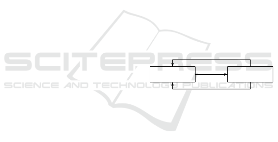
Reinforcement Learning: is a method allowing an

autonomous agent to adapt his behavior during the ex-

ecution by updating his model.

Agent Environnement

Action

Feedback

State

Figure 1: Representation of reinforcement learning.

The agent starts with an initial model to compute

the policy to be followed during the execution. The

execution of this initial policy leads to feed-backs

from the environment, particularly the reward ob-

tained after the execution. The obtained feed-backs

allow us to update the model and to compute a new

policy.

Many algorithms have been developed such as Q-

learning (Watkins and Dayan, 1992), temporal dif-

ference TD(λ) or SARSA (Sutton and Barto, 1998).

Our approach uses a reinforcement learning similar to

techniques with a reward function update procedure.

TAMER (Knox and Stone, 2008): is an algorithm

used to train an agent with deterministic actions. It

uses an MDP model without a reward function. An

operator will train the robot by sending a positive or a

negative signal H to the agent. This algorithm differs

with what we want to do, because the agent needs to

be trained before executing the algorithm. Moreover,

ECTA 2016 - 8th International Conference on Evolutionary Computation Theory and Applications

194

we are not trying to train an agent, but to learn his pol-

icy to adapt the observer behavior. We can, however,

adapt the model by sending a positive reward for each

state reached by the agent.

TAMER&RL(Knox and Stone, 2010)(Knox and

Stone, 2012) is the computation between TAMER and

a Reinforcement Learning method. It allows us to re-

duce the time of training.

Imitation Learning. Is a training method. The

agent ﬁrst observes an operator to complete the mis-

sion, and learns the policy with this observation.

Many algorithms exist for imitation learning and pre-

sented in (He et al., 2012).

The idea of this algorithm is similar to our idea.

However, the agent tries to learn the Master (leader in

our case) policy to imitate him. In our approach we

learn the Leader policy not to imitate him but to com-

pute a best-response to better coordinate with him.

4 OUR APPROACH

The policy prediction is mainly based on series of pol-

icy estimation followed by a policy update. The ob-

served agents are semi-autonomous or tele-operated.

Consequently, the MDP model of the observed agent

is already deﬁned, even in the tele-operation case.

First, we compute an optimal policy from their MDP

model as an approximate initial policy and then we

update it during the execution of this policy using the

reinforcement learning techniques. Indeed, we, ini-

tially, assume that the Leader (the semi-autonomous

agent) follows an optimal policy and when observ-

ing its behavior, we get information on the executed

action, the rewarded value and the state o = (a,r,s).

When the observation o shows that the executed ac-

tion a is different from the expected action π(s)), the

autonomous agent (follower) updates the predicted

policy π considering this deviation. The policy update

to predict a new policy is based on three methods.

During the execution of the mission, the agent

may choose different action from the estimated pol-

icy, due to the operators hesitations, preferences or

perception. These changes are stored in a history H.

Let H

(t) and H

(t) be respectively the history of the

state and the action of the last operations up to time

t. These histories represent the feed-backs of the en-

vironment during the last t operations which will be

considered for updating the initial policy π

init

. To this

end, we will present three update methods to generate

a new estimated policy π from π

init

and (H

(t), H

(t)).

The ”Force” Method. The idea behind this

method is to update the current estimated policy by

modifying some actions at some states using the his-

tory. Indeed, this method is a ”forcing” approach

where actions performed at some states in the last op-

erations are introduced in the current estimated pol-

icy when a deviation from the estimated policy is ob-

served. We assign, then, states in H

(t) with actions

in H

(t), and then we compute the optimal actions

for the other states not concerned with the changes to

generate a new estimated policy. More formally :

new











∀0 ≤ k ≤ t,s

∈ H

(t) and a

∈ H

(t) :

new

) = a

∀s /∈ H

(t) : π

new

(s) =

argmax

a∈A

∑

∈S

p(s

|s,a)(r(s

|s,a) +V

∗

))

The ”Learn” Method. Instead of the previous

method where we change actions at some states of

the current policy, this method is based on adapting

the reward function to consider the preferences of the

operator observed from the last previous operations.

To this end, we assume that the operator acts to reach

the desired and preferred states. More formally, we

will deﬁne X as the set of n variables composing the

states of the agent. Each of these variables x

∈ X are

deﬁned in a domain D

. The idea is to assign a reward

to each variable which may interest the operator, and

apply a cost for each variable which could be unpleas-

ant to him. Then, by changing the reward function,

the policy might evolve consequently. Let x

(s) be the

value of the variable x

from the state s, and let Q

the preference function for the operator for the vari-

able x

. Q

(v) is the reward function to the variable x

when it takes the value v. Consequently, Q

(s)) is

the reward attributed to the variable x

from the state

s. Initially, every variables Q

are set to 0, and c is

the constant value to add to the reward function. The

constant c might be chosen by considering the values

on the reward function. With a high value, each action

executed different from the estimated action will have

a high impact on the policy update.

Algorithm 1 allows us to assign, to each successor

state reachable from the deviation of the original pol-

icy, a reward according to the probability to reach it

from the deviation. In the same way, we assign a cost

for each state which should be reached by the current

policy. To generate the new policy, we then compute a

new reward function r

, with the equation 3. We then

generate a new policy with the MDP hS,A, p,r

|s,a) = r(s

|s,a) +

∑

∈X

)) (3)

Non-optimal Semi-autonomous Agent Behavior Policy Recognition

195

Algorithm 1: Reward update.

1 for t ∈ [0..k] do

2 if H

(t) 6= π(H

(t)) then

3 for s

successor of (H

(t),H

(t)) do

4 for i ∈ [0..n] do

5 Q

)) = Q

)) +

p(s

(t),H

(t)) × c;

6 for s

successor of (H

(t),π(H

(t)) do

7 for i ∈ [0..n] do

8 Q

)) = Q

)) −

p(s

(t),π(H

(t)) × c;

Generalization: Consider a factored representation of

states with n variables such that s = (v

,...,v

), as

depicted in Fig.2. The expected action at s is π(s)

leading to s

= (v

,...,v

n−1

) while the semi-

autonomous agent executes action a(s) leading to

= (v

,...,v

n−1

). Let’s consider that s

dif-

fers from s

at the ﬁrst and the last variables. v

6= v

and v

6= v

while the other variables are identical.

s = hv

, v

, . . . , v

′

= hv

′

, v

′

, . . . , v

′

i s

′′

= hv

′′

, v

′

, . . . , v

′′

π(s) a(s)

Figure 2: Representation of a derivation.

Learn method will increase the reward of all states

s = (v

,∗, . . . , ∗, ∗) and s = (∗,∗,...,∗,v

) represent-

ing the preferred states of the operator and will re-

duce the reward of states s = (v

,∗,...,∗,∗) and s =

(∗,∗,...,∗,v

) representing unpleasant states by as-

suming that the operator prefers a(s) to π(s) to reach

preferred states with features v

and v

rather than the

ones with features v

and v

Reward increase

(s = hv

,∗,...,∗i) = r

(s) + Q

)

...

(s = h∗, ∗, . . . , v

i) = r

(s) + Q

)

Reward decrease

(s = hv

,∗,...,∗i) = r

(s) + Q

)

...

(s = h∗, ∗, . . . , v

i) = r

(s) + Q

)

This algorithm estimates the operator preferences

according to the concerned states. Meanwhile, when

a deviation occurs, the reward update is propagated

into the all state space and will affect the behavior

policy of the semi-autonomous agent. This latter may

overreact to derivations leading to the generation of

more prediction errors than corrections, and then may

create an unstable prediction process.

The ”Dist” Method. This method is similar to the

”Learn” Method by reducing the impact of the local

updates. To this end, we should restrict the propa-

gation to some states which are close to the updated

state. To assess the closeness, we deﬁne the distance

between two states in an MDP as the number of vari-

ables different from each other. Each state reach-

able by the predicted action will receive a cost and

reversely. however, each state reachable by the pre-

dicted action will get a reward corresponding to the

value of the parameters with reward for the observed

action, in the condition that the distance between this

state and another reachable by the observed action is

less or equals to a threshold δ.

Generalization: We consider, at time t, that the oper-

ator derives from the predicted policy.

= hv

, v

, . . . , v

= hv

′

, v

′

, . . . , v

i s

= hv

′

, v

′

, . . . , v

′

h1, 0, . . . , 1i

π(s) a(s)

Figure 3: Calculation of a distance.

The distance between s

and s

is 2 because

,...,v

) differs from (v

,...,v

) on vari-

ables v

and v

. For example, if δ = 1, considering s

as a state reachable by the observed action and s

as a

state reachable by the predicted action, we will obtain

the following modiﬁcations on the reward function:

) = r(s

) +

∑

i=1

)

) = r(s

) +

∑

i=1

)

= hv

,...,v

i) = r(s

) + Q

)

...

= hv

,...,v

i) = r(s

) + Q

)

= hv

,...,v

i) = r(s

) + Q

)

...

= hv

,...,v

i) = r(s

) + Q

)

The ﬁrst two equations are about decreasing the

reward for the states reachable by the estimated action

and increasing the reward for the ones reachable by

the executed action. The next two equations represent

the increase of states closed to the ones reachable by

the executed actions, oppositely to the last two ones.

5 EXPERIMENTS

We develop experiments to show the efﬁciency and

the impact of the operator hesitation on the prediction

to show the robustness of the methods to the operator

mistakes. We also develop experiments on the im-

pact of delta in the Dist method to assess their perfor-

mances. We consider two kinds of environments of

ECTA 2016 - 8th International Conference on Evolutionary Computation Theory and Applications

196

the site surveillance, an indoor environments where

the robots evolve in a restricted space and an outdoor

environment where the space is open and there is a

limited impact of locality. We consider that in these

environments the areas have three levels of lighting

from very bright to dark leading the agent to select

the right actions (using the right sensor) to better be-

have. An optimal policy allows the agent to use the

best action at a state according to the lighting level

and when the agent uses an action different from the

optimal one, it gets a cost. The mission of the agent is

to start at a location and targets a new one for surveil-

lance. We formalize the tele-operation process of the

agent by an MDP. To simulate the operator prefer-

ences, we will force the MDP policy to choose one

action on speciﬁc states (to force the agent to follow

or to avoid a path) before generating the optimal pol-

icy. To formalize the hesitation, we deﬁne probabilis-

tic policies, in which the operator selects probabilisti-

cally some actions at some states. During the execu-

tion, we used the learning methods described above

to predict the behavior of the semi-autonomous agent,

and compare the prediction results. To evaluate their

efﬁciency, we consider the number of prediction er-

rors made by each prediction method.

We also compare these methods with an adapted

TAMER&RL (TAMER combined with SARSA(λ)),

on which the learning algorithm will receive a re-

ward for each action dictated by the operator to the

semi-autonomous agent. TAMER&RL was conﬁg-

ured with the Table 1. ”Learn” and ”Dist” methods

are conﬁgured with the following parameters c = 3

and k = 10.

Table 1: Conﬁguration of TAMER&RL.

Parameter value

TAMER

α 0.2

SARSA-LAMBDA:

α 0.8

ε 0

γ 1

λ 1

β 0.98

5.1 Results in Indoor Environments

During the experiments, we recorded the number of

prediction errors during the 50 executions of the mis-

sions. In this experiment, we compare the algorithms

in different situations: deterministic and stochastic

actions, operator doesn’t hesitate representing an ex-

pert and self-control operator, operator hesitates fre-

quently representing a non-expert operator and oper-

ator hesitates sometimes representing an expert oper-

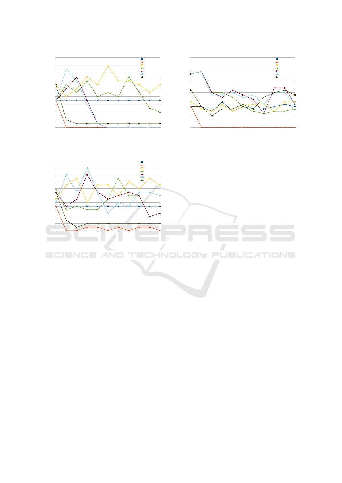
0 5 10 15 20 25 30 35 40 45 49

Autonomous

FORCE

LEARN

Dist-0

Dist-1

Dist-2

TAMER&RL

Execution Number

Number of prediction errors

Figure 4: Results with no hesitation.

ator, but can make some mistakes in some stressed

situations.

Without Hesitation: Expert and Self-control Op-

erator. Fig.4 represents the number of prediction

errors according to the number of the mission execu-

tion. The autonomous curve corresponds to the opti-

mal policy of an autonomous agent, without learning

during the execution. This algorithm is used here to

show the impact of learning. Note that ”Dist-i” corre-

sponds to the ”Dist” method, with δ=i.

We can see that almost all curves converge to 0,

which means that almost all algorithms learn correctly

the agent policy. The only exception is TAMER&RL,

which keeps one prediction error over the time. How-

ever, it’s under the autonomous curve. TAMER&RL

starts with a high number of prediction error because

the algorithm starts the learning from scratch without

considering the past mission executions. ”Force” and

”Learn” curves are similar in this case, and they con-

verge quickly. However, we can see that ”Dist” meth-

ods are not stable, in the beginning, but they converge

and ﬁnd the agent policy after some periods of time.

To conclude, our methods outperform TAMER&RL

and converge more quickly.

0 5 10 15 20 25 30 35 40 45 49

Autonomous

FORCE

LEARN

Dist-0

Dist-1

Dist-2

TAMER&RL

Execution Number

Number of prediction errors

Figure 5: Results with 30% hesitation on some states.

Non-optimal Semi-autonomous Agent Behavior Policy Recognition

197

With 30% Hesitation: Non-expert Operator. We

can see in Fig.5 that the prediction methods are

more unstable during the whole execution, except

for the ”Learn”, ”Force” and TAMER&RL methods.

”Learn” and ”Force” curves are similar and converge,

but they still get few errors in some cases. How-

ever, these algorithms learn globally the agent policy.

”Dist” methods are more unstable than before, and get

a lot of prediction errors at the beginning. The only

one who seems to be stable is for δ = 0. The others

seem to be close to the agent policy, but each variation

on the agent policy generates many perturbations on

the prediction. The ”Learn” method does not present

a high number of mistakes, but he is much perturbed

by hesitations than the ”Force” or the TAMER&RL

methods. The ”Force” method gets an error every

time the agent changes the action of the policy at a

state. Otherwise he is the most efﬁcient.

Impact of Stochastic Transitions. For the experi-

ments, we ﬁrst used deterministic actions to compare

the results with TAMER&RL, because this method

needs deterministic transitions. We repeated the ex-

periments to see the impact of stochastic transitions,

to analyze the robustness of the different algorithms.

To do so, we adapted the TAMER&RL policy by con-

sidering the stochastic transition function.

0 5 10 15 20 25 30 35 40 45 49

Autonomous

FORCE

LEARN

Dist-0

Dist-1

Dist-2

TAMER&RL

Execution Number

Number of prediction errors

Figure 6: Results without hesitation, but with stochastic ac-

tions.

We can see in Fig.6 that TAMER&RL does not

present the same results with stochastic transitions.

Indeed, TAMER&RL seems inappropriate for learn-

ing if transitions are not deterministic. All our

approaches outperform TAMER&RL. On the other

hand, without hesitation, ”Dist” methods seems to be

more efﬁcient with stochastic transitions than deter-

ministic ones. The reason may be that each transition

leads to several states, so the Dist methods learn on

more states, but still locally.

0 5 10 15 20 25 30 35 40 45 49

Autonomous

FORCE

LEARN

Dist-0

Dist-1

Dist-2

TAMER&RL

Execution Number

Number of prediction errors

Figure 7: Results with 30% hesitation, but with stochastic

actions.

On Fig.7, we can see that with a high rate of hes-

itations, every method get unstable. This is not sur-

prising because it implies a lot of execution changes.

For each time a new state is reached, each time the

pilot policy can derive from the autonomous policy.

It implies a lot of policy modiﬁcations to learn. The

”Force” and the ”Learn” methods seem predict well.

However, ”Dist” methods and TAMER&RL are to-

tally unstable and does not predict well. ”Dist” meth-

ods seem to learn after the 20th execution. This is

due to the fact that a lot of new states were reached

between the 35th and the 40th, since every method

started to get prediction errors at this moment.

Nevertheless the hesitation is implemented by

choosing between two actions randomly. Moreover,

the agent policy is generated with transition functions

adapted with hesitation, but an operator would not

know when he will have doubts, and doesn’t know his

probability to choose an action at this moment. Fur-

thermore, the hesitations rate may decease over the

time since the operator learns also from his previous

experiments of the mission.

5.2 Results in Outdoor Environment

We developed a new serie of experiments in outdoor

environment where the branching factor in the state

space is high.

With 0% Hesitation: Expert and Self-control Op-

erator. We can see in Fig.8 that the ”Force” method

is still better than the others including TAMER&RL.

”Learn” method is not as efﬁcient as in restricted

space, and is less efﬁcient than the autonomous pol-

icy. The reason is that in such environments the

branching factor is high and the number of states

reachable from the current one is high. Then, updat-

ing the operator preferences in all the state space may

ECTA 2016 - 8th International Conference on Evolutionary Computation Theory and Applications

198

0 5 10 15 20 25 30 35 40 45 49

Autonomous

FORCE

LEARN

Dist-0

Dist-1

Dist-2

TAMER&RL

Execution Number

Number of prediction errors

Figure 8: Results with 0% hesitation on an open space, with

deterministic actions.

0 5 10 15 20 25 30 35 40 45 49

Autonomous

FORCE

LEARN

Dist-0

Dist-1

Dist-2

TAMER&RL

Execution Number

Number of prediction errors

Figure 9: Results with 30% hesitation in an open determin-

istic space.

impact all the policy, while in indoor environments

the state space is restricted. By limiting the learning

ﬁeld, ”Dist” method avoids this effect and learns the

agent policy, except with a δ=0.

With 30% Hesitation: Non-expert Operator.

With hesitation, on Fig.9, almost no method, excepted

TAMER&RL and ”Force” method, can predict cor-

rectly the agent policy. ”Dist” methods show best re-

sults than ”Learn”, but they are still less efﬁcient than

the autonomous policy. Indeed, when the operator is

not stable is difﬁcult to learn from this behavior the

operator preferences while maintaining a policy with

local update is better because it’s still not far from the

optimal policy which in such cases are suitable.

Impact of Stochastic Transitions. With stochastic

transitions on Fig.10, as expected, TAMER&RL can-

not predict anything, and Force method remain efﬁ-

cient. The other policy predictions are unstable, and

less efﬁcient than the optimal policy, excepted Dist-0.

0 5 10 15 20 25 30 35 40 45 49

Autonomous

FORCE

LEARN

Dist-0

Dist-1

Dist-2

TAMER&RL

Execution Number

Number of prediction errors

Figure 10: Results without hesitation in an open space with

stochastic transitions.

5.3 Synthesis

The table 2 shows the efﬁciency of each method in

different cases. ++ means that the method learns

quickly the policy. + Means that the algorithm learns

the policy, but the convergence is slow, and − means

that the algorithm is not efﬁcient. However, ”Force”

is efﬁcient in any situation. ”Learn” is efﬁcient only

with restricted environments, such as indoor ones.

TAMER&RL is efﬁcient on deterministic transitions,

but there exist a more efﬁcient alternative in any sit-

uation. ”Dist” method is much efﬁcient without hes-

itations. Also, in indoor environments, it works bet-

ter with stochastic transitions. However, in outdoor

environments, the algorithm is efﬁcient only when in

deterministic transition cases.

6 CONCLUSION

We addressed in this paper the problem of estimating

the policy of a semi-autonomous agent where this lat-

ter could follow a policy other than the optimal one.

To this end, we develop an approach based on ini-

tializing the policy to the optimal one and then up-

date this policy according to the observed behavior

and the operator actions. We propose three update

methods to predict the next behavior of the system by

estimating the new policy. These methods are based

on the history of the last operations to change the cur-

rent policy or to update the reward function. We dis-

tinguished between a method propagating the reward

update in the whole state space and a method restrict-

ing the propagation to subspace by deﬁning a notion

of distance among states.

The experiments show satisfying and promising

results and showing a robustness to the operator mis-

takes in indoor environments, except for the ”Dist”

Non-optimal Semi-autonomous Agent Behavior Policy Recognition

199

Table 2: Efﬁciency of prediction methods, considering the situation.

environment Indoor Outdoor

transitions Det. Stoc. Det. Stoc.

hesitation no yes no yes no yes no yes

Force ++ ++ ++ ++ ++ ++ ++ ++

Learn ++ ++ ++ + − − − −

Dist + + ++ − ++ − − −

TAMER&RL + + − − + + − −

method who learns mistakes and take a lot of time

before learning. TAMER&RL is much stable with

deterministic actions than ”Force” and ”Learn” meth-

ods, but less efﬁcient. In stochastic transition cases,

TAMER&RL is outperformed by every other method.

In outdoor environment, ”Dist” method seems to be

much adapted, contrary to ”Learn” method.

In short-term, we will integrate our methods in a

multi-robot system, developed in a national project,

on the sensitive site surveillance example where a

robot is tele-operated by a professional operator and

the other should predict its policy and compute a co-

ordinated policy to head the same destination.

ACKNOWLEDGEMENT

We would like to thank the DGA (General Direction

of Arming), Dassault-Aviation and Nexter Robotics

for their ﬁnancial participation for these results.

REFERENCES

Abdel-Illah Mouaddib, L. J. and Zilberstein, S. (2015).

Handling advice in mdps for semi-autonomous sys-

tems. In ICAPS Woskhop on Planning and Robotics

(PlanRob), pages 153–160.

He, H., Eisner, J., and Daume, H. (2012). Imitation learning

by coaching. In Pereira, F., Burges, C., Bottou, L., and

Weinberger, K., editors, Advances in Neural Informa-

tion Processing Systems 25, pages 3149–3157. Curran

Associates, Inc.

uttenrauch, H. and Severinson Eklundh, K. (2006). Be-

yond usability evaluation: Analysis of human-robot

interaction at a major robotics competition. Interac-

tion Studies, 7(3):455–477.

Knox, W. and Stone, P. (2008). Tamer: Training an agent

manually via evaluative reinforcement. In Develop-

ment and Learning, 2008. ICDL 2008. 7th IEEE In-

ternational Conference on, pages 292–297.

Knox, W. B. and Stone, P. (2010). Combining manual

feedback with subsequent MDP reward signals for re-

inforcement learning. In Proc. of 9th Int. Conf. on

Autonomous Agents and Multiagent Systems (AAMAS

2010).

Knox, W. B. and Stone, P. (2012). Reinforcement learning

with human and mdp reward. In Proceedings of the

11th International Conference on Autonomous Agents

and Multiagent Systems (AAMAS 2012).

Monderer, D. and Shapley, L. S. (1996). Potential games.

Games and economic behavior, 14(1):124–143.

Nair, R., Tambe, M., Yokoo, M., Pynadath, D. V., and

Marsella, S. (2003). Taming decentralized pomdps:

Towards efﬁcient policy computation for multiagent

settings. In IJCAI-03, Proceedings of the Eighteenth

International Joint Conference on Artiﬁcial Intelli-

gence, Acapulco, Mexico, August 9-15, 2003, pages

705–711.

Panagou, D. and Kumar, V. (2014). Cooperative Visibility

Maintenance for Leader-Follower Formations in Ob-

stacle Environments. Robotics, IEEE Transactions on,

30(4):831–844.

Paruchuri, P., Pearce, J. P., Marecki, J., Tambe, M., Or-

donez, F., and Kraus, S. (2008). Playing games

for security: An efﬁcient exact algorithm for solving

bayesian stackelberg games. In Proceedings of the 7th

International Joint Conference on Autonomous Agents

and Multiagent Systems - Volume 2, AAMAS ’08,

pages 895–902, Richland, SC. International Founda-

tion for Autonomous Agents and Multiagent Systems.

Pashenkova, E., Rish, I., and Dechter, R. (1996). Value it-

eration and policy iteration algorithms for markov de-

cision problem. In AAAI’96: Workshop on Structural

Issues in Planning and Temporal Reasoning. Citeseer.

Puterman, M. L. (1994). Markov Decision Processes: Dis-

crete Stochastic Dynamic Programming. John Wiley

& Sons, Inc., New York, NY, USA, 1st edition.

Shiomi, M., Sakamoto, D., Kanda, T., Ishi, C. T., Ishiguro,

H., and Hagita, N. (2008). A semi-autonomous com-

munication robot: a ﬁeld trial at a train station. In

Proceedings of the 3rd ACM/IEEE International Con-

ference on Human Robot Interaction, pages 303–310,

New York, NY, USA. ACM.

Sigaud, O. and Buffet, O. (2010). Markov Decision Pro-

cesses in Artiﬁcial Intelligence. Wiley-ISTE.

Sutton, R. S. and Barto, A. G. (1998). Introduction to Re-

inforcement Learning. MIT Press, Cambridge, MA,

USA.

Vorobeychik, Y., An, B., and Tambe, M. (2012). Adver-

sarial patrolling games. In Proceedings of the 11th

International Conference on Autonomous Agents and

Multiagent Systems - Volume 3, AAMAS ’12, pages

1307–1308, Richland, SC. International Foundation

for Autonomous Agents and Multiagent Systems.

Watkins, C. and Dayan, P. (1992). Q-learning. Machine

Learning, 8(3-4):279–292.

ECTA 2016 - 8th International Conference on Evolutionary Computation Theory and Applications

200