Model-Intersection Problems with Existentially Quantiﬁed Function

Variables: Formalization and a Solution Schema

Kiyoshi Akama

and Ekawit Nantajeewarawat

Information Initiative Center, Hokkaido University, Sapporo, Hokkaido, Japan

Computer Science, Sirindhorn International Institute of Technology, Thammasat University, Pathumthani, Thailand

Keywords:

Model-Intersection Problem, Extended Clause, Function Variable, Equivalent Transformation.

Abstract:

Built-in constraint atoms play a very important role in knowledge representation and are indispensable for

practical applications. It is very natural to use built-in constraint atoms together with user-deﬁned atoms when

formalizing logical problems using ﬁrst-order formulas. In the presence of built-in constraint atoms, however,

the conventional Skolemization in general preserves neither the satisﬁability nor the logical meaning of a

given ﬁrst-order formula, motivating us to step outside the conventional Skolemization and the usual space of

ﬁrst-order formulas. We propose general solutions for proof problems and query-answering (QA) problems

on ﬁrst-order formulas possibly with built-in constraint atoms. We map, by using new meaning-preserving

Skolemization, all proof problems and all QA problems, preserving their answers, into a new class of model-

intersection (MI) problems on an extended clause space, where clauses are in a sense “higher-order” since they

may contain not only built-in constraint atoms but also function variables. We propose a general schema for

solving this class of MI problems by equivalent transformation (ET), where problems are solved by repeated

simpliﬁcation using ET rules. The correctness of this solution schema is shown. Since MI problems in this

paper form a very large class of logical problems, this theory is also useful for inventing solutions for many

classes of logical problems.

1 INTRODUCTION

A proof problem is a “yes/no” problem; it is con-

cerned with checking whether or not one given logical

formula entails another given logical formula. For-

mally, a proof problem is a pair hE

i, where E

and E

are ﬁrst-order formulas, and the answer to this

problem is deﬁned to be “yes” if E

is a logical con-

sequence of E

, and it is deﬁned to be “no” otherwise.

A proof problem hE

i is solved (Chang and Lee,

1973; Robinson, 1965) by (i) constructing the formula

E = (E

∧ ¬E

), since the unsatisﬁability of E means

that the answer of this proof problem is “yes”, (ii)

conversion of E into a set Cs of clauses using the con-

ventional Skolemization (Chang and Lee, 1973; Fit-

ting, 1996), (iii) transformation of the clause set Cs

by the resolution and factoring inference rules, and

(iv) determining the answer by checking whether an

empty clause can be obtained, i.e., if an empty clause

is obtained, then Cs is unsatisﬁable and the answer to

the proof problem is “yes”. This solution relies on

the preservation of satisﬁability. The conversion of

E into Cs using the conventional Skolemization pre-

serves the satisﬁability of E. Transformation of Cs

by using resolution and factoring also preserves the

satisﬁability of Cs.

A query-answering problem (QA problem) on

clauses is a pair hCs,ai, where Cs is a set of clauses

and a is a user-deﬁned query atom. The answer to

a QA problem hCs,ai is deﬁned as the set of all

ground instances of a that are logical consequences

of Cs. Characteristically, a QA problem is an “all-

answers ﬁnding” problem, i.e., all ground instances of

a given query atom satisfying the requirement above

are to be found. In our previous work (Akama and

Nantajeewarawat, 2015a), for solving proof prob-

lems on ﬁrst-order formulas and QA problems on

clauses, these problems are transformed into model-

intersection problems (MI problems) on the conven-

tional clause space. Such a MI problem is a pair

hCs,ϕi, where Cs is a set of clauses and ϕ is a map-

ping, called an exit mapping, used for constructing

the output answer from the intersection of all models

of Cs. More formally, the answer to a MI problem

hCs,ϕi is ϕ(

Models(Cs)), where Models(Cs) is the

set of all models of Cs and

Models(Cs) is the inter-

Akama, K. and Nantajeewarawat, E.

Model-Intersection Problems with Existentially Quantiﬁed Function Variables: Formalization and a Solution Schema.

DOI: 10.5220/0006056800520063

In Proceedings of the 8th International Joint Conference on Knowledge Discovery, Knowledge Engineering and Knowledge Management (IC3K 2016) - Volume 2: KEOD, pages 52-63

ISBN: 978-989-758-203-5

section of all elements of Models(Cs). Note that, in

this theory, an interpretation is a set of ground user-

deﬁned atoms, which is similar to a Herbrand inter-

pretation (Chang and Lee, 1973; Fitting, 1996). Since

each element of Models(Cs) is a set of ground user-

deﬁned atoms, we can take the intersection of all ele-

ments of it.

In this paper, we consider ﬁrst-order formulas that

possibly includes built-in constraint atoms. The set of

all such formulas is denoted by FOL

. Built-in con-

straint atoms play a crucial role in knowledge repre-

sentation and are essential for practical applications.

One of the objectives of this paper is to propose gen-

eral solutions for proof problems and QA problems

on FOL

, which are large problem classes that have

never been solved fully so far. The classical theorem-

proving theory motivates us to transform proof prob-

lems and QA problems on FOL

into MI problems

on clauses by the conventional Skolemization (Chang

and Lee, 1973; Fitting, 1996). However, satisﬁabil-

ity preservation of a formula does not generally hold

for formulas in FOL

(Akama and Nantajeewarawat,

2015b). The conventional Skolemization, therefore,

does not provide a transformation process towards

correct solutions for proof problems and QA prob-

lems on FOL

Meaning-preserving Skolemization (MPS) was

invented(Akama and Nantajeewarawat, 2008; Akama

and Nantajeewarawat, 2011) to overcome the difﬁcul-

ties caused by the conventional Skolemization. MPS

preserves the logical meanings of ﬁrst-order formu-

las (and, thus, also preserves their satisﬁability) even

when they include built-in constraint atoms. Con-

ventional clauses should be extended in order that

all ﬁrst-order formulas in FOL

can be equivalently

converted by MPS. An extended clause may contain

function variables and atoms of a special kind called

func-atoms. The set of all extended clauses is called

ECLS

This paper introduces a model-intersection prob-

lem (MI problem) on this extended space, which is

a pair hCs,ϕi, where Cs is a set of extended clauses

and ϕ is an exit mapping. The set of all MI problems

on the extended clauses constitutes a very large class

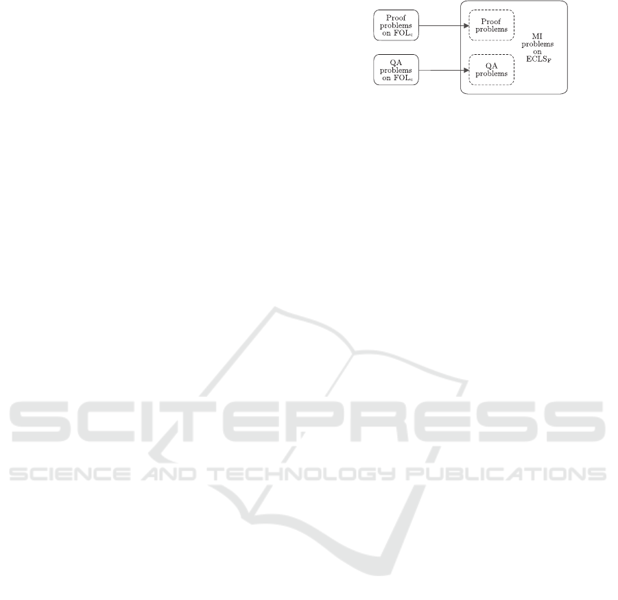
of problems and is of great importance. As outlined

by Fig. 1, all proof problems and all QA problems

on FOL

are mapped, preserving their answers, into

MI problems on ECLS

. By solving MI problems on

ECLS

, we solve proof problems and QA problems

on FOL

. We propose a general schema for solving

MI problems on ECLS

by equivalent transformation

(ET), where problems are solved by repeated problem

simpliﬁcation using ET rules.

The class of MI problems established in this pa-

Figure 1: MI-problem-centered view of logical problems.

per is the largest and the ﬁrst one that enables struc-

tural embedding of the full class of proof problems

on FOL

and the full class of QA problems on FOL

The class of MI problems considered in our previous

work (Akama and Nantajeewarawat, 2015a) involves

only usual clauses (with no function variable being

allowed) and is not sufﬁcient for dealing with proof

problems and QA problems on FOL

entirely.

The rest of the paper is organized as follows: Sec-

tion 2 deﬁnes extended clauses and ECLS

, and intro-

duces meaning-preserving Skolemization. Section 3

formalizes MI problems on extended clauses and de-

scribes how QA problems and proof problems can be

convertedinto MI problems. Section 4 presents a gen-

eral schema for solving MI problems by ET. Section 5

demonstrates an application of the general schema.

Section 6 concludes the paper.

The notation that follows holds thereafter. Given

a set A, pow(A) denotes the power set of A. Given

two sets A and B, Map(A,B) denotes the set of all

mappings from A to B, and for any partial mapping

f from A to B, dom( f) denotes the domain of f, i.e.,

dom( f) = {a | (a ∈ A) & ( f(a) is deﬁned)}.

2 AN EXTENDED CLAUSE SPACE

2.1 User-deﬁned Atoms, Built-in

Constraint Atoms, and func-Atoms

An extended formula space is introduced, which con-

tains three kinds of atoms, i.e., user-deﬁned atoms,

built-in constraint atoms, and func-atoms. A user-

deﬁned atom takes the form p(t

,...,t

), where p is a

user-deﬁned predicate and the t

are usual terms. Sup-

posing that teach, St, and FM are user-deﬁned pred-

icates, teach(john,ai), St(paul), and FM(x) are user-

deﬁned atoms (cf. Fig. 3 in Section 5). A built-in con-

straint atom, also simply called a constraint atom or

a built-in atom, takes the form c(t

,...,t

), where c is

a predeﬁned constraint predicate and the t

are usual

terms. Typical examples of built-in constraint atoms

are eq(x,x) and neq(1,2), where eq and neq are prede-

ﬁned constraint predicates that stand for “equal” and

“not equal,” respectively. (No built-in constraint atom

Model-Intersection Problems with Existentially Quantiﬁed Function Variables: Formalization and a Solution Schema

appears in Fig. 3.) Let A

be the set of all user-deﬁned

atoms, G

the set of all ground user-deﬁned atoms, A

the set of all constraint atoms, and G

the set of all

ground constraint atoms.

A func-atom (Akama and Nantajeewarawat,2011)

is an expression of the form func( f,t

,...,t

n+1

where f is either an n-ary function constant or an n-

ary function variable, and the t

are usual terms. For

example, supposing that f

is a unary function vari-

able, func( f

,x,y) is a func-atom (cf. the clauses C

andC

in Fig. 3). A func-atom func( f,t

,...,t

n+1

)

is ground if f is a function constant and the t

are

ground usual terms.

There are two types of variables: usual variables

and function variables. (In Fig. 3, x, y, z, and w are

usual variables, while f

is a function variable.) A

function variable is instantiated into a function con-

stant or a function variable, but not into a usual term.

Let FVar be the set of all function variables and

FCon the set of all function constants. A substitu-

tion for function variables is a mapping from FVar to

FVar∪ FCon. Each n-ary function constant is associ-

ated with a mapping from G

to G

, where G

denotes

the set of all usual ground terms.

2.2 Extended Clauses

User-deﬁned atoms and built-in constraint atoms are

used in usual clauses, which are extended by allow-

ing func-atoms to appear in their right-hand sides. An

extended clause C is a formula of the form

,...,a

← b

,...,b

,...,f

where each of a

,...,a

,...,b

is a user-deﬁned

atom or a built-in constraint atom, f

,...,f

are func-

atoms, and m, n, and p are non-negative integers.

All usual variables occurring in C are implicitly uni-

versally quantiﬁed and their scope is restricted to

the extended clause C itself. The sets {a

,...,a

}

and {b

,...,b

,...,f

} are called the left-hand side

and the right-hand side, respectively, of the extended

clause C, and are denoted by lhs(C) and rhs(C), re-

spectively. Let userLhs(C) denote the number of

user-deﬁned atoms in the left-hand side of C. When

userLhs(C) = 0, C is called a negative extended

clause. When userLhs(C) = 1,C is called an extended

deﬁnite clause. When userLhs(C) > 1, C is called a

multi-head extended clause.

When no confusion is caused, an extended clause,

a negative extended clause, an extended deﬁnite

clause, and a multi-head extended clause are also

called a clause, a negative clause, a deﬁnite clause,

and a multi-head clause, respectively.

Let DCL denote the set of all extended deﬁnite

clauses with no constraint atom in their left-hand

sides. Given a deﬁnite clause C ∈ DCL, the user-

deﬁned atom in lhs(C) is called the head of C, de-

noted by head(C), and the set rhs(C) is called the

body of C, denoted by body(C).

2.3 An Extended Clause Space

A conjunction of a ﬁnite or inﬁnite number of ex-

tended clauses is used for knowledge representation

and also for computation. As usual, such a conjunc-

tion is usually dealt with by regarding it as a set of

(extended) clauses. The set of all extended clauses is

denoted by ECLS

. The extended clause space in this

paper is the powerset of ECLS

Let Cs be a set of extended clauses. Implicit ex-

istential quantiﬁcations of function variables and im-

plicit clause conjunction are assumed in Cs. Func-

tion variables in Cs are all existentially quantiﬁed and

their scope covers all clauses in Cs. With occurrences

of function variables, clauses in Cs are connected

through shared function variables. After instantiating

all function variables in Cs into function constants,

clauses in the instantiated set are totally separated.

2.4 Conversion of First-order Formulas

into Sets of Extended Clauses

Semantically, an extended clause corresponds to a

disjunction of extended literals, and a set of ex-

tended clauses corresponds to an extended conjunc-

tive normal form. After explaining the limitations

of the conventional Skolemization, conversion of a

ﬁrst-order formula in FOL

into a set of extended

clauses in ECLS

by meaning-preserving Skolemiza-

tion (Akama and Nantajeewarawat, 2008; Akama and

Nantajeewarawat, 2011) is introduced.

2.4.1 Conventional Skolemization

In the conventional proof theory, a ﬁrst-order formula

is usually converted into a conjunctive normal form

in the usual ﬁrst-order formula space. The conver-

sion involves removal of existential quantiﬁcations by

Skolemization (Chang and Lee, 1973; Fitting, 1996),

i.e., by replacement of an existentially quantiﬁed vari-

able with a Skolem term determined by its relevant

quantiﬁcation structure. Let CSK(E) denote the set

of usual clauses obtained by applying this conversion

to a ﬁrst-order formula E.

The conventional Skolemization, however, does

not generally preserve the logical meaning of a ﬁrst-

order formula in FOL

, nor the satisﬁability thereof.

This is precisely shown by Theorem 1 below. Given a

ﬁrst-order formula E in FOL

and a set Cs of extended

KEOD 2016 - 8th International Conference on Knowledge Engineering and Ontology Development

clauses in ECLS

, let Models(E) and Models(Cs) de-

note the set of all models of E and that of all models

of Cs, respectively.

Theorem 1.

1. There are a ﬁrst-order formula E in FOL

and a

clause set Cs ⊆ ECLS

such that CSK(E) = Cs

and Models(E) 6= Models(Cs).

2. There are a ﬁrst-order formula E in FOL

and a

clause set Cs ⊆ ECLS

such that CSK(E) = Cs,

Models(E) 6= ∅, and Models(Cs) = ∅.

Proof: Assume that:

• noteq is a predicate for built-in constraint atoms

and for any ground terms t

and t

, noteq(t

) is

true iff t

6= t

• F

, F

, and F

are the ﬁrst-order formulas in

FOL

given by:

: ∀x∀y∀z : [(hasChild(x,y) ∧ hasChild(x,z)

∧ noteq(y,z)) → TaxCut(x)]

: hasChild(Peter,Paul)

: ∃x : hasChild(Peter, x)

: ¬(∃x : TaxCut(x))

Consider a ﬁrst-order formula E = F

∧ F

Obviously, Models(E) 6= ∅ and a model of E is

{hasChild(Peter,Paul)}. Let CSK(E) = Cs. Then

Cs consists of the following clauses, where f is a new

constant:

TaxCut(x) ← hasChild(x,y),hasChild(x,z),

noteq(y,z)

hasChild(Peter,Paul) ←

hasChild(Peter, f) ←

← TaxCut(x)

Since f is a constant and noteq(Paul, f) is true, the

clause set Cs has no model, i.e., Models(Cs) = ∅.

Hence Results 1 and 2 of this theorem hold.

2.4.2 Meaning-preserving Skolemization

In order to transform a ﬁrst-order formula equiv-

alently into a set of extended clauses, meaning-

preserving Skolemization was invented in (Akama

and Nantajeewarawat, 2008; Akama and Nantajee-

warawat, 2011). Let MPS(E) denote the set of

extended clauses resulting from applying meaning-

preserving Skolemization to a given ﬁrst-order for-

mula E in FOL

. MPS(E) is obtained from E by re-

peated subformula transformationand conversioninto

a clausal form. Consider, for example, the ﬁrst-order

formula E in the proof of Theorem 1. MPS(E) is

the clause set Cs

′

consisting of the following extended

clauses, where h is a 0-ary function variable:

TaxCut(x) ← hasChild(x,y),hasChild(x,z),

noteq(y,z)

hasChild(Peter,Paul) ←

hasChild(Peter,x) ← func(h,x)

← TaxCut(x)

An algorithm for computing MPS(E) was given

in (Akama and Nantajeewarawat, 2011). Each trans-

formation used by this algorithm preserves the logical

meaning of an input formula. As a result, the next the-

orem is obvious.

Theorem 2. Let E be a ﬁrst-order formula in FOL

and Cs ⊆ ECLS

. If MPS(E) = Cs, then

1. Models(E) = Models(Cs), and

2. Models(E) = ∅ iff Models(Cs) = ∅.

2.5 Interpretations and Models

A state of the world is represented by a set of true

ground atoms in G

. A logical formula is used to

impose a constraint on possible states of the world.

Hence, an interpretation is a subset of G

. A ground

user-deﬁned atom g is true under an interpretation I

iff g belongs to I. Unlike ground user-deﬁned atoms,

the truth values of ground constraint atoms are prede-

termined independently of interpretations. Let TCON

denote the set of all true ground constraint atoms,

i.e., a ground constraint atom g is true iff g ∈ TCON.

A ground func-atom func( f,t

,...,t

n+1

) is true iff

f(t

,...,t

) = t

n+1

A ground clause C = (a

,...,a

← b

,...,b

...,f

) ∈ ECLS

is true under an interpretation I (in

other words, I satisﬁes C) iff at least one of the fol-

lowing conditions is satisﬁed:

1. There exists i ∈ {1,...,m} such that a

∈ I ∪

TCON.

2. There exists i ∈ {1,...,n} such that b

/∈ I ∪

TCON.

3. There exists i ∈ {1,..., p} such that f

is false.

An interpretation I is a model of a clause set Cs ⊆

ECLS

iff there exists a substitution σ for function

variables that satisﬁes the following conditions:

1. All function variables occurring in Cs are instan-

tiated by σ into function constants.

2. For any clause C ∈ Cs and any substitution θ for

usual variables, if Cσθ is a ground clause, then

Cσθ is true under I.

Let Models be a mapping that associates with each

clause set the set of all of its models, i.e., Models(Cs)

is the set of all models of Cs for any Cs ⊆ ECLS

Model-Intersection Problems with Existentially Quantiﬁed Function Variables: Formalization and a Solution Schema

The standard semantics is taken in this theory in

the sense that all models of a formula are considered

instead of speciﬁc ones, such as those considered in

the minimal model semantics (Clark, 1978; Lloyd,

1987), which underlies deﬁnite logic programming,

and in the stable model semantics (Gelfond and Lifs-

chitz, 1988; Gelfond and Lifschitz, 1991), which un-

derlies answer set programming.

3 MODEL-INTERSECTION

PROBLEMS

3.1 Model Intersection is Important

Assume that a person A and a person B are interested

in knowing which atoms in G

are true and which

atoms in G

are false. They want to know the un-

known set G of all true ground atoms. Due to short-

age of knowledge, A still cannot identify one unique

subset of G

as the state of the world. The person A

can only limit possible subsets of true atoms by spec-

ifying a subset Gs of pow(G

). The unknown set G of

all true atoms belongs to Gs.

One way for A to inform this knowledge to B com-

pactly is to send to B a clause set Cs such that Gs ⊆

Models(Cs). Receiving Cs, B knows that Models(Cs)

includes all possible intended sets of ground atoms,

i.e., G ∈ Models(Cs). As such, B can know that each

ground atom outside

Models(Cs) is false, i.e., for

any g ∈ G

, if g /∈

Models(Cs), then g /∈ G. The

person B can also know that each ground atom in

Models(Cs) is true, i.e., for any g ∈ G

, if g ∈

Models(Cs), then g ∈ G. This shows the impor-

tance of calculating

Models(Cs).

3.2 Model-Intersection (MI) Problems

on the Extended Clause Space

It is natural for us to seek information about the model

intersection of given knowledge, which motivates us

to introduce a new class of logical problems.

A model-intersection problem (MI problem) on

ECLS

is a pair hCs,ϕi, where Cs ⊆ ECLS

and ϕ

is a mapping from pow(G

) to some set W. The map-

ping ϕ is called an exit mapping. The answer to this

problem, denoted by ans

(Cs,ϕ), is deﬁned by

ans

(Cs,ϕ) = ϕ(

Models(Cs)),

where

Models(Cs) is the intersection of all models

of Cs. Note that when Models(Cs) is the empty set,

Models(Cs) = G

Example 1. Consider the Oedipus puzzle described

in (Baader et al., 2007). Oedipus killed his father,

married his mother Iokaste, and had children with her,

among them Polyneikes. Polyneikes also had chil-

dren, among them Thersandros, who is not a patri-

cide. The problem is to ﬁnd all persons who have a

patricide child who has a non-patricide child.

Assume that (i) “oe,” “io,” “po” and “th” stand, re-

spectively, for Oedipus, Iokaste, Polyneikes and Ther-

sandros, (ii) for any terms t

and t

, isCh(t

) de-

notes “t

is a child of t

,” and (iii) for any termt, pat(t)

denotes “t is a patricide” and prob(t) denotes “t is an

answer to this puzzle.” To formalize this puzzle, let

consist of the following seven clauses:

isCh(oe,io) ← isCh(po,io) ←

isCh(po,oe) ← isCh(th,po) ←

pat(oe) ← ← pat(th)

prob(x), pat(y) ← isCh(z,x),pat(z),isCh(y,z)

Let ϕ

be deﬁned by ϕ

(G) = {x | prob(x) ∈ G} for

any G ⊆ G

. Then hCs

,ϕ

i is an MI problem repre-

senting this puzzle.

Example 2. Consider a problem of ﬁnding all lists

obtained by concatenating [1,2,3] with [4,5]. Let Cs

consist of the following clauses:

app([],x,x) ←

app([w|x],y,[w|z]) ← app(x,y, z)

ans(x) ← app([1, 2, 3],[4,5],x)

Let ϕ

be deﬁned by ϕ

(G) = {x | ans(x) ∈ G} for

any G ⊆ G

. This problem is then formalized as the

MI problem hCs

,ϕ

Example 3. Consider the “tax-cut” problem dis-

cussed in (Motik et al., 2005). This problem is to

ﬁnd all persons who can have discounted tax, with

the knowledge consisting of the following statements:

(i) Any person who has two children or more can

get discounted tax. (ii) Men and women are not the

same. (iii) It is false that a person is not the same

as himself/herself. (iv) A person’s mother is always

a woman. (v) Peter has a child, who is someone’s

mother. (vi) Peter has a child named Paul. (vii) Paul

is a man. These statements are represented by the fol-

lowing eight extended clauses:

TaxCut(x) ←hasChild(x,y), hasChild(x,z),

notSame(y,z)

notSame(x,y) ← Man(x),Woman(y)

← notSame(x,x)

Woman(x) ← motherOf(x,y)

hasChild(Peter,x) ← func( f

,x)

motherOf(x,y) ← func( f

,x), func( f

,y)

hasChild(Peter,Paul) ←

KEOD 2016 - 8th International Conference on Knowledge Engineering and Ontology Development

Man(Paul) ←

The ﬁfth and the sixth clauses together represent the

ﬁfth statement (i.e., “Peter has a child, who is some-

one’s mother”), where f

and f

are 0-ary function

variables. Let Cs

consist of the above eight clauses.

Let ϕ

be deﬁned by ϕ

(G) = {x | TaxCut(x) ∈ G}

for any G ⊆ G

. The “tax-cut” problem is then for-

mulated as the MI problem hCs

,ϕ

Example 4. Consider the “Dreadsbury Mansion

Mystery” problem, which was given by Len Schubelt

and can be described as follows: Someone who lives

in Dreadsbury Mansion killed Aunt Agatha. Agatha,

the butler, and Charles live in Dreadsbury Mansion,

and are the only people who live therein. A killer

always hates his victim, and is never richer than his

victim. Charles hates no one that Aunt Agatha hates.

Agatha hates everyone except the butler. The butler

hates everyone not richer than Aunt Agatha. The but-

ler hates everyone Agatha hates. No one hates every-

one. The problem is to ﬁnd who is the killer.

Assume that neq is a predeﬁned binary constraint

predicate and for any ground usual terms t

and t

neq(t

) is true iff t

6= t

. The background knowl-

edge of this mystery is formalized as a set Cs

consist-

ing of the following clauses, where the constants A,

B, C, and D denote “Agatha,” “the butler,” “Charles,”

and “Dreadsbury Mansion,” respectively, f

is a 0-ary

function variable, and f

is a unary function variable:

live(x,D) ← func( f

,x)

kill(x,A) ← func( f

,x)

← live(x,D),neq(x,A),neq(x,B),neq(x,C)

live(A,D) ←

live(B,D) ←

live(C,D) ←

hate(x,y) ← kill(x,y)

← kill(x,y), richer(x, y)

← hate(A,x),hate(C,x),live(x, D)

hate(A,x) ← neq(x,B),live(x, D)

richer(x,A),hate(B,x) ←

hate(B,x) ← hate(A,x)

← hate(x,y),func( f

,x,y),live(x,D)

live(y,D) ← live(x,D),func( f

,x,y)

killer(x) ← kill(x,A)

Let ϕ

be deﬁned by ϕ

(G) = {x | killer(x) ∈ G} for

any G ⊆ G

. This problem is then represented as the

MI problem hCs

,ϕ

Example 5. Let an exit mapping ϕ

be given as fol-

lows: For any G ⊆ G

, ϕ

(G) = “yes” if G = G

and ϕ

(G) = “no” otherwise. Referring to the clause

sets Cs

–Cs

in Examples 1–4, we illustrate that proof

problems can be represented as MI problems as fol-

lows:

• Letting Cs

= Cs

∪{(← prob(io))}, the MI prob-

lem hCs

,ϕ

i represents the problem of proving

whether prob(io) is true.

• Letting Cs

= Cs

∪ {(← ans([1,2,3,4,5]))}, the

MI problem hCs

,ϕ

i represents the problem of

proving whether the resulting list is [1,2,3,4,5].

• Letting Cs

= Cs

∪ {(← TaxCut(x))}, the MI

problem hCs

,ϕ

i represents the problem of

proving whether someone gets discounted tax.

• Letting Cs

= Cs

∪ {(← killer(A))}, the MI

problem hCs

,ϕ

i represents the problem of

proving whether Agatha killed herself.

3.3 Conversion of Query-Answering

(QA) Problems into MI Problems

A query-answeringproblem (QA problem) on FOL

a pair hE,ai, where E is a closed ﬁrst-order formula in

FOL

and a is a user-deﬁned atom in A

. Let S be the

set of all substitutions for usual variables. The answer

to a QA problem hE,ai, denoted by ans

(E, a), is

deﬁned by

ans

(E, a) = {aθ | (θ ∈ S) & (aθ ∈ G

) & (E |= aθ)}.

In logic programming (Lloyd, 1987), a problem

represented by a pair of a set of deﬁnite clauses and a

query atom has been intensively discussed. In the de-

scription logic (DL) community (Baader et al., 2007),

a class of problems formulated as conjunctions of

DL-based axioms and assertions together with query

atoms has been discussed (Tessaris, 2001). These two

problem classes can be formalized as subclasses of

QA problems considered in this paper.

Theorem 3. For any closed ﬁrst-order formula E ∈

FOL

and any a ∈ A

ans

(E, a) = rep(a) ∩ (

Models(E)),

where rep(a) denotes the set of all ground instances

of a.

Proof: Let E be a closed ﬁrst-order formula in

FOL

and a ∈ A

. By the deﬁnition of |=, for any

ground atom g ∈ G

, E |= g iff g ∈

Models(E).

Then

ans

(E, a)

= {aθ | (θ ∈ S ) & (aθ ∈ G

) & (E |= aθ)}

= {g | (θ ∈ S) & (g = aθ) & (g ∈ G

) & (E |= g)}

= {g | (g ∈ rep(a)) & (E |= g)}

= {g | (g ∈ rep(a)) & (g ∈ (

Models(E)))}

= rep(a) ∩ (

Models(E)).

Model-Intersection Problems with Existentially Quantiﬁed Function Variables: Formalization and a Solution Schema

Theorem 4 below shows that a QA problem on

FOL

can be converted into a MI problem on ECLS

Theorem 4. Let E be a ﬁrst-order formula in FOL

and a ∈ A

. Let Cs ⊆ ECLS

. If Models(E) =

Models(Cs), then

ans

(E, a) = ans

(Cs∪{(p(x

,...,x

) ← a)},ϕ

where p is a predicate that appears in neither Cs nor

a, the arguments x

,...,x

are all the mutually differ-

ent variables occurring in a, and for any G ⊆ G

(G) = {aθ | (θ ∈ S) & (p(x

,...,x

)θ ∈ G)}.

Proof: Assume that Models(E) = Models(Cs).

Then

ans

(E, a)

= (by Theorem 3)

= rep(a) ∩ (

Models(E))

= rep(a) ∩ (

Models(Cs))

= (by the deﬁnition of ϕ

)

= ϕ

(

Models(Cs∪ {(p(x

,...,x

) ← a)}))

= ans

(Cs∪ {(p(x

,...,x

) ← a)},ϕ

3.4 Conversion of Proof Problems into

MI Problems

A proof problem is a pair hE

i, where E

and E

are ﬁrst-order formulas in FOL

, and the answer to

this problem, denoted by ans

), is deﬁned by

ans

) =



“yes” if E

|= E

“no” otherwise.

It is well known that that E

is a logical consequence

of E

iff E

∧ ¬E

is unsatisﬁable (i.e., E

∧ ¬E

has

no model) (Chang and Lee, 1973; Fitting, 1996). As

a result, ans

) can be equivalently deﬁned by

ans

) =



“yes” if Models(E

∧ ¬E

) = ∅,

“no” otherwise.

Theorem 5 below shows that a proof problem can

be converted into a MI problem on ECLS

Theorem 5. Let hE

i be a proof problem, where

and E

are ﬁrst-order formulas in FOL

. Let

Cs ⊆ ECLS

. Let ϕ

: pow(G

) → {“yes”,“no”} be

deﬁned by: for any G ⊆ G

(G) =



“yes” if G = G

“no” otherwise.

If the conditions Models(E

∧ ¬E

) = ∅ and

Models(Cs) = ∅ are equivalent, then ans

) =

ans

(Cs,ϕ

Proof: Assume that Models(E

∧ ¬E

) = ∅ iff

Models(Cs) = ∅. Let b be a ground user-deﬁnedatom

that is not an instance of any user-deﬁned atom occur-

ring in Cs. If m is a model of Cs, then m−{b} is also a

model of Cs. Obviously, m− {b} 6= G

. Therefore, (i)

if Models(Cs) 6= ∅, then

Models(Cs) 6= G

, and (ii)

if Models(Cs) = ∅, then

Models(Cs) =

{} = G

Two cases are considered:

1. Suppose that Models(E

∧ ¬E

) = ∅. Conse-

quently, Models(Cs) = ∅. So

Models(Cs) =

, and, therefore, ans

(Cs,ϕ

) = “yes”.

2. Suppose that Models(E

∧¬E

) 6= ∅. In this case,

Models(Cs) 6= ∅, and, thus,

Models(Cs) 6= G

So ans

(Cs,ϕ

) = “no”.

Hence ans

) = ans

(Cs,ϕ

4 SOLVING MI PROBLEMS BY

EQUIVALENT

TRANSFORMATION

A general schema for solving MI problems based on

equivalent transformation (ET) is formulated and its

correctness is shown (Theorem 10).

4.1 Preservation of Partial Mappings

and Equivalent Transformation

Terminologies such as preservation of partial map-

pings and equivalent transformation are deﬁned in

general below. They will be used with a speciﬁc class

of partial mappings called target mappings, which

will be introduced in Section 4.2.

Assume that X and Y are sets and f is a par-

tial mapping from X to Y. For any x,x

′

∈ dom( f),

transformation of x into x

′

is said to preserve f iff

f(x) = f(x

′

). For any x,x

′

∈ dom( f), transformation

of x into x

′

is called equivalent transformation (ET)

with respect to f iff the transformation preserves f,

i.e., f(x) = f(x

′

Let F be a set of partial mappings from a set X

to a set Y. Given x,x

′

∈ X, transformation of x into

′

is called equivalent transformation (ET) with re-

spect to F iff there exists f ∈ F such that the trans-

formation preserves f. A sequence [x

,...,x

] of

elements in X is called an equivalent transformation

sequence (ET sequence) with respect to F iff for any

i ∈ {0, 1, . . . , n − 1}, transformation of x

into x

i+1

ET with respect to F. When emphasis is placed on

the initial element x

and the ﬁnal element x

, this se-

quence is also referred to as an ET sequence from x

to x

KEOD 2016 - 8th International Conference on Knowledge Engineering and Ontology Development

4.2 Target Mappings

We introduce the concept of target mapping, which is

useful to devise equivalent transformation (ET) rules

in the ECLS

space (Theorem 9) or to construct an

answer mapping (Theorem 8) for determining an an-

swer from the ﬁnal state of computation.

The answer to a MI problem hCs,ϕi is determined

uniquely by Models(Cs) and ϕ. MI problems can thus

be transformed into simpler forms by ET preserving

the mapping Models.

Simpliﬁcation of MI problems using ET preserv-

ing the mapping Models can be extended by consider-

ing additional partial mappings. A new classof partial

mappings, called GSETMAP, will be deﬁned below.

Deﬁnition 1. GSETMAP is the set of all partial map-

pings from pow(ECLS

) to pow(pow(G

)).

As deﬁned in Section 2.5, Models(Cs) is the set

of all models of Cs for any Cs ⊆ ECLS

. Since a

model is a subset of G

, Models is regarded as a total

mapping from pow(ECLS

) to pow(pow(G

)). Since

a total mapping is also a partial mapping, the map-

ping Models is a partial mapping from pow(ECLS

)

to pow(pow(G

)), i.e., it is an element of GSETMAP.

A partial mapping M in GSETMAP is of par-

ticular interest if

M(Cs) =

Models(Cs) for any

Cs ∈ dom(M). Such a partial mapping is called a tar-

get mapping.

Deﬁnition 2. A partial mapping M ∈ GSETMAP is a

target mapping iff for any Cs ∈ dom(M),

M(Cs) =

Models(Cs).

It is obvious that:

Theorem 6. The mapping Models is a target map-

ping.

The next theorem provides a sufﬁcient condition

for a mapping in GSETMAP to be a target mapping.

Theorem 7. Let M ∈ GSETMAP. M is a target map-

ping if the following conditions are satisﬁed:

1. M(Cs) ⊆ Models(Cs) for any Cs ∈ dom(M).

2. For any Cs ∈ dom(M) and any m

∈ Models(Cs),

there exists m

∈ M(Cs) such that m

⊆ m

Proof: Assume that Conditions 1 and 2 above

are satisﬁed. Let Cs ∈ dom(M). By Condition 1,

M(Cs) ⊇

Models(Cs). We show that

M(Cs) ⊆

Models(Cs) as follows: Assume that g ∈

M(Cs).

Let m

∈ Models(Cs). By Condition 2, there exists

∈ M(Cs) such that m

⊆ m

. Since g ∈

M(Cs),

g belongs to m

. So g ∈ m

. Since m

is any arbitrary

element of Models(Cs), g belongs to

Models(Cs).

It follows that

M(Cs) =

Models(Cs). Hence M is

a target mapping.

4.3 Answer Mappings

A set of problems that can be solved at low cost is

useful to provide a desirable ﬁnal destination for ET

computation. It can also be speciﬁed as a partial map-

ping that is preserved by ET transformation. Such a

speciﬁcation is useful to invent and to justify new ET

transformation. This motivates the concept of answer

mapping, which is formalized below.

Deﬁnition 3. Let W be a set. A partial mapping A

from

pow(ECLS

) × Map(pow(G

),W)

to W is an answer mapping iff for any hCs, ϕi ∈

dom(A), ans

(Cs,ϕ) = A(Cs,ϕ).

If M is a target mapping, then M can be used for

constructing answer mappings.

Theorem 8. Let M be a target mapping. Suppose that

A is a partial mapping such that

• dom(M) = {x | hx,yi ∈ dom(A)}, and

• for any hCs,ϕi ∈ dom(A),

A(Cs,ϕ) = ϕ(

M(Cs)).

Then A is an answer mapping.

Proof: Let hCs, ϕi ∈ dom(A). Since dom(M) =

{x | hx,yi ∈ dom(A)}, Cs belongs to dom(M). Since

M is a target mapping,

M(Cs) =

Models(Cs). So

ans

(Cs,ϕ) = ϕ(

Models(Cs))

= ϕ(

M(Cs))

= A(Cs,ϕ).

Thus A is an answer mapping.

4.4 ET Steps and ET Rules

A schema for solving MI problems based on equiva-

lent transformation (ET) preserving answers is formu-

lated. The notions of preservation of answers/target

mappings, ET with respect to answers/target map-

pings, and an ET sequence are obtained by special-

izing the general deﬁnitions in Section 4.1.

Let STATE be the set of all MI problems. Elements

of STATE are called states.

Deﬁnition 4. Let hS,S

′

i ∈ STATE × STATE. hS, S

′

i is

an ET step iff if S = hCs,ϕi and S

′

= hCs

′

,ϕ

′

i, then

ans

(Cs,ϕ) = ans

(Cs

′

,ϕ

′

Model-Intersection Problems with Existentially Quantiﬁed Function Variables: Formalization and a Solution Schema

Deﬁnition 5. A sequence [S

,...,S

] of ele-

ments of STATE is an ET sequence iff for any i ∈

{0,1, . . . , n − 1}, hS

i+1

i is an ET step.

The role of ET computation constructing [S

...,S

] is to start with S

and to reach S

from which

the answer to the given problem can be easily com-

puted.

The concept of ET rule on STATE is deﬁned by:

Deﬁnition 6. An ET rule r on STATE is a partial

mapping from STATE to STATE such that for any

S ∈ dom(r), hS,r(S)i is an ET step.

We also deﬁne ET rules on pow(ECLS

) as fol-

lows:

Deﬁnition 7. An ET rule r with respect to a target

mapping M is a partial mapping from pow(ECLS

) to

pow(ECLS

) such that for any Cs∈ dom(r), M(Cs) =

M(r(Cs)).

We can construct an ET rule on STATE from an

ET rule with respect to a target mapping.

Theorem 9. Assume that M is a target mapping and

r is an ET rule with respect to M. Suppose that ¯r is a

partial mapping from STATE to STATE such that

• dom(r) = {x | hx, yi ∈ dom(¯r)}, and

• ¯r(S) = hr(Cs),ϕi if S = hCs,ϕi ∈ dom(¯r).

Then ¯r is an ET rule on STATE.

Proof: Assume that S ∈ dom(¯r). Then there exist

a clause set Cs and an exit mapping ϕ such that S =

hCs,ϕi and Cs ∈ dom(r). For such Cs and ϕ,

ans

(Cs,ϕ) = ϕ(

Models(Cs))

= (since M is a target mapping)

= ϕ(

M(Cs))

= (since M(Cs) = M(r(Cs)))

= ϕ(

M(r(Cs)))

= (since M is a target mapping)

= ϕ(

Models(r(Cs)))

= ans

(r(Cs), ϕ).

Since S = hCs,ϕi and ¯r(S) = hr(Cs),ϕi, hS, ¯r(S)i is

an ET step. Hence ¯r is an ET rule on STATE.

4.5 Correct Solutions based on ET

Rules

Given a set Cs of extended clauses and an exit map-

ping ϕ, the MI problem hCs,ϕi can be solved as fol-

lows:

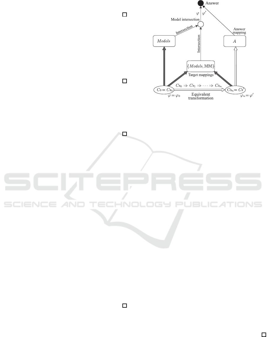
1. Let A be an answer mapping.

Figure 2: Target mappings and answer mappings yield

many correct computation paths.

2. Prepare a set R of ET rules on STATE.

3. Take S

such that S

= hCs,ϕi to start computa-

tion from S

4. Construct an ET sequence [S

,...,S

] by applying

ET rules in R, i.e., for each i ∈ {0,1, . . .,n − 1},

i+1

is obtained from S

by selecting and applying

∈ R such that S

∈ dom(r

) and r

) = S

i+1

5. Assume that S

= hCs

,ϕ

i. If the computation

reaches the domain of A, i.e., hCs

,ϕ

i ∈ dom(A),

then compute the answer by using the answer

mapping A, i.e., output A(Cs

,ϕ

The answer to the MI problem hCs,ϕi, i.e.,

ans

(Cs,ϕ) = ϕ(

Models(Cs)), can be directly ob-

tained by the computation shown in the leftmost path

in Fig. 2. Instead of taking this computation path, the

above solution takes a different one, i.e., the lowest

path (from Cs to Cs

′

) followed by the rightmost path

(through A) in Fig. 2.

The selection of r

in R at Step 4 is nondeterminis-

tic and there may be many possible computation paths

for each MI problem. Every output computed by us-

ing any arbitrary computation path is correct.

Theorem 10. When an ET sequence starting from

= hCs,ϕi reaches S

in dom(A), the above proce-

dure gives the correct answer to hCs,ϕi.

Proof: Since [S

,...,S

] is an ET sequence,

ans

(Cs,ϕ) = ans

(Cs

,ϕ

). Since A is an an-

swer mapping, ans

(Cs

,ϕ

) = A(Cs

,ϕ

). Hence

ans

(Cs,ϕ) = A(Cs

,ϕ

KEOD 2016 - 8th International Conference on Knowledge Engineering and Ontology Development

: FM(x) ← FP(x) C

: FP(john) ←

: FP(mary) ← C

: teach(john,ai) ←

: St(paul) ← C

: AC(ai) ←

: Tp(kr) ← C

: Tp(lp) ←

: curr(x,z) ← exam(x,y), subject(y,z),St(x),

Co(y),Tp(z)

: mdt(x,y) ← curr(x,z),expert(y,z), St(x),Tp(z),

FP(y),AC(w),teach(y,w)

: mdt(x,y) ← St(x),NFP(y)

: exam(paul,ai) ← C

: subject(ai,kr) ←

: subject(ai,lp) ← C

: expert(john,kr) ←

: expert(mary,lp) ←

: AC(x) ← teach(mary,x)

: ← AC(x),BC(x)

: AC(x),BC(x) ← Co(x)

: Co(x) ← AC(x)

: Co(x) ← BC(x)

: FP(x) ← NFP(x)

: ← NFP(x),teach(x,y),Co(y)

: teach(x,y), NFP(x) ← FP(x),func( f

,x,y)

: Co(y),NFP(x) ← FP(x), func( f

,x,y)

Figure 3: Background knowledge for the mdt problem on

ECLS

5 EXAMPLE

5.1 Problem Description

The clauses in Fig. 3 are obtained from the “may-

do-thesis” problem (for short, the mdt problem) given

in (Donini et al., 1998) with some modiﬁcation. All

atoms appearing in Fig. 3 belong to A

. The unary

predicates NFP, FP, FM, Co, AC, BC, St, and Tp

denote “non-teaching full professor,” “full profes-

sor,” “faculty member,” “course,” “advanced course,”

“basic course,” “student,” and “topic,” respectively.

The clauses C

–C

together provide the conditions

for a student to do his/her thesis with a professor,

where mdt(s, p), curr(s,t), expert(p,t), exam(s,c),

and subject(c,t) are intended to mean “s may do

his/her thesis with p,” “s studied t in his/her curricu-

lum,” “p is an expert in t,” “s passed the exam of c,”

and “c covers t,” respectively, for any student s, any

professor p, any topic t, and any course c.

Suppose that we want to ﬁnd all professors with

whom paul may do his thesis. This problem is formu-

lated as a MI problem hCs,ϕi, where Cs consists of

the clauses C

–C

in Fig. 3 and ϕ is deﬁned by: for

any G ⊆ G

ϕ(G) = {x | mdt(paul,x) ∈ G}.

: teach(john,ai) ←

: AC(ai) ←

: AC(x) ← teach(mary,x)

: ← AC(x),BC(x)

: AC(x),BC(x) ← Co(x)

: Co(x) ← AC(x)

: Co(x) ← BC(x)

: ← NFP(x),teach(x,y),Co(y)

: mdt(paul,mary) ← AC(x), teach(mary, x),

Co(ai)

: mdt(paul,john) ← AC(x),teach(john,x),

Co(ai)

: mdt(paul,x) ← NFP(x)

: teach(mary,x), NFP(mary) ← func( f

,mary,x)

: teach(john,x), NFP(john) ← func( f

,john,x)

: Co(x),NFP(mary) ← func( f

,mary,x)

: Co(x),NFP(john) ← func( f

,john,x)

Figure 4: Clauses obtained by application of ET rules.

How to compute the answer to this MI problem using

many kinds of clause transformation rules is demon-

strated in Section 5.2.

5.2 ET Computation

The clause set Cs consisting of C

–C

given in Sec-

tion 5.1 (Fig. 3) is transformed as follows:

• By (i) unfolding using the deﬁnitions of the pred-

icates FP, Tp, curr, subject, expert, St, and exam,

(ii) removing these deﬁnitions along with the def-

inition of FM using deﬁnite-clause removal, (iii)

removal of valid clauses, and (iv) removal of

subsumed clauses, the clauses C

–C

are trans-

formed into the clauses C

–C

in Fig. 4.

• Side-change transformation for NFP enables (i)

unfolding using the deﬁnition of Co, (ii) elimi-

nation of this deﬁnition using deﬁnite-clause re-

moval, and (iii) removal of valid clauses. By such

side-change transformation followed by transfor-

mation of these three types, C

–C

are trans-

formed into the clauses C

–C

in Fig. 5.

• Side-change transformation for BC enables un-

folding using the deﬁnition of AC. By (i) un-

folding, (ii) deﬁnite-clause removal, (iii) removal

of duplicate atoms, (iv) removal of valid clauses,

and (v) removal of subsumed clauses, C

–C

are

transformed into C

–C

in Fig. 6.

• By (i) unfolding using the deﬁnition of teach, (ii)

deﬁnite-clause removal, (iii) removal of duplicate

atoms, (iv) removal of valid clauses, and (v) re-

moval of subsumed clauses, C

–C

are trans-

formed into C

–C

in Fig. 7.

Model-Intersection Problems with Existentially Quantiﬁed Function Variables: Formalization and a Solution Schema

: teach(john,ai) ←

: AC(ai) ←

: AC(x) ← teach(mary,x)

: ← AC(x),BC(x)

: mdt(paul,mary) ← AC(x),teach(mary,x),

func( f

,mary,ai),

notNFP(mary)

: mdt(paul,mary) ← AC(x),teach(mary,x),

func( f

,john,ai),

notNFP(john)

: mdt(paul,mary) ← AC(x),teach(mary, x),BC(ai)

: mdt(paul,mary) ← AC(x),teach(mary, x),AC(ai)

: mdt(paul,john) ← AC(x),teach(john,x),

func( f

,mary,ai),

notNFP(mary)

: mdt(paul,john) ← AC(x),teach(john,x),

func( f

,john,ai),

notNFP(john)

: mdt(paul,john) ← AC(x),teach(john, x),BC(ai)

: mdt(paul,john) ← AC(x),teach(john, x),AC(ai)

: mdt(paul,x),notNFP(x) ←

: teach(mary,x) ← func( f

,mary, x),

notNFP(mary)

: teach(john,x) ← func( f

,john,x),

notNFP(john)

: notNFP(x) ← teach(x,y),func( f

,mary,y),

notNFP(mary)

: notNFP(x) ← teach(x,y),func( f

,john,y),

notNFP(john)

: notNFP(x) ← teach(x,y),BC(y)

: notNFP(x) ← teach(x,y),AC(y)

: AC(x),BC(x) ← func( f

,mary, x),

notNFP(mary)

: AC(x),BC(x) ← func( f

,john,x),

notNFP(john)

Figure 5: Clauses obtained by application of ET rules.

• By deﬁnite-clause removal for notBC, C

–C

are transformed into C

–C

in Fig. 8.

• Application of the resolution rule to C

and C

followed by removal of independent func-atoms

and removal of duplicated atoms, yields the clause

in Fig. 9. By removal of subsumed clauses,

and C

are removed. By deﬁnite clause re-

moval, C

is removed. Then C

–C

are trans-

formed into C

–C

in Fig. 9.

As a result, the MI problem hCs,ϕi in Sec-

tion 5.1 is transformed equivalently into the MI prob-

lem h{C

},ϕi. Hence

ans

(Cs,ϕ)

= ans

({C

},ϕ)

= ϕ(

Models({C

}))

= ϕ({mdt(paul,mary),mdt(paul,john)})

= {mary,john}.

: teach(john,ai) ←

: notBC(ai) ←

: notBC(x) ← teach(mary,x)

: notNFP(x),notBC(y) ← teach(x,y)

: notNFP(x) ← teach(x,y),func( f

,john,y),

notNFP(john)

: notNFP(x) ← teach(x,y),func( f

,mary,y),

notNFP(mary)

: mdt(paul,mary) ← teach(mary,x)

: mdt(paul,john) ← teach(john,x),

teach(mary,x)

: mdt(paul,john) ← teach(john,ai)

: mdt(paul,john) ← teach(john,x),

func( f

,mary,x),

notNFP(mary), notBC(x)

: mdt(paul,john) ← teach(john,x),

func( f

,john,x),

notNFP(john),notBC(x)

: mdt(paul,x),notNFP(x) ←

: teach(mary,x) ← func( f

,mary,x),

notNFP(mary)

: teach(john,x) ← func( f

,john,x),

notNFP(john)

: notNFP(x) ← teach(x,ai)

: notNFP(x) ← teach(x,y),teach(mary,y)

Figure 6: Clauses obtained by application of ET rules.

: notBC(x) ← func( f

,mary,x),notNFP(mary)

: mdt(paul,x),notNFP(x) ←

: notBC(ai) ←

: mdt(paul,john) ←

: mdt(paul,mary) ← func( f

,mary,x),

notNFP(mary)

: notNFP(john) ←

Figure 7: Clauses obtained by application of ET rules.

: mdt(paul,x),notNFP(x) ←

: mdt(paul,john) ←

: mdt(paul,mary) ← func( f

,mary, x),

notNFP(mary)

: notNFP(john) ←

Figure 8: Clauses obtained by application of ET rules.

: mdt(paul,mary) ←

: mdt(paul,john) ←

Figure 9: Clauses obtained by application of ET rules.

6 CONCLUSIONS

We have deﬁned a class of model-intersection (MI)

problems on extended clauses possibly with con-

straint atoms and func-atoms, each of which is a pair

of a set Cs of extended clauses and an exit mapping

KEOD 2016 - 8th International Conference on Knowledge Engineering and Ontology Development

used for constructing the output answer from the in-

tersection of all models of Cs. Many logical prob-

lems, including proof problems and query-answering

(QA) problems, can be transformed into MI problems

preserving their answers. The theory in this paper

therefore providesa foundation for many kinds of log-

ical problem solving.

We introduced the concepts of target mapping and

answer mapping, which are useful for inventing many

kinds of ET rules for solving MI problems on ex-

tended clauses. The proposed solution schema for MI

problems comprises the following steps: (i) formal-

ize a given problem as a MI problem or map it into a

MI problem, (ii) prepare ET rules from answers/target

mappings, (iii) construct an ET sequence preserving

answers/target mappings, and (iv) compute the an-

swer by using some answer mapping (possibly con-

structed on some target mapping).

Many logical problems, among others, all proof

problems and all QA problems on FOL

, are mapped,

by using new meaning-preserving Skolemization

(Akama and Nantajeewarawat, 2011), into MI prob-

lems with function variables, and solved by ET com-

putation proposed in this paper. When only con-

ventional clauses without function variables are used,

meaning-preserving Skolemization is impossible. In

the presence of built-in constraint atoms, the classical

theory, which uses the conventional Skolemization,

cannot guarantee the correctness of the conversion of

logical formulas into clauses.

The ET-based solution method together with

meaning-preserving Skolemization is very general

and fundamental, since any combination of ET steps

forms correct computation and the correctness of the

method for a very large class of problems has been

shown in this paper. By its generality, the theory de-

veloped in this paper makes clear a fundamental and

central structure of representation and computation

for logical problem solving.

ACKNOWLEDGEMENTS

This research was partially supported by JSPS KAK-

ENHI Grant Numbers 25280078 and 26540110.

REFERENCES

Akama, K. and Nantajeewarawat, E. (2008). Meaning-

Preserving Skolemization on Logical Structures. In

Proceedings of the 9th International Conference

on Intelligent Technologies, pages 123–132, Samui,

Thailand.

Akama, K. and Nantajeewarawat, E. (2011). Meaning-

Preserving Skolemization. In Proceedings of the 3rd

International Conference on Knowledge Engineering

and Ontology Development, pages 322–327, Paris,

France.

Akama, K. and Nantajeewarawat, E. (2015a). A General

Schema for Solving Model-Intersection Problemson a

Specialization System by Equivalent Transformation.

In Proceedings of the 7th International Joint Confer-

ence on Knowledge Discovery, Knowledge Engineer-

ing and Knowledge Management (IC3K 2015), Vol-

ume 2: KEOD, pages 38–49, Lisbon, Portugal.

Akama, K. and Nantajeewarawat, E. (2015b). Function-

variable Elimination and Its Limitations. In Pro-

ceedings of the 7th International Joint Conference

on Knowledge Discovery, Knowledge Engineering

and Knowledge Management (IC3K 2015), Volume 2:

KEOD, pages 212–222, Lisbon, Portugal.

Baader, F., Calvanese, D., McGuinness, D. L., Nardi, D.,

and Patel-Schneider, P. F., editors (2007). The De-

scription Logic Handbook. Cambridge University

Press, second edition.

Chang, C.-L. and Lee, R. C.-T. (1973). Symbolic Logic and

Mechanical Theorem Proving. Academic Press.

Clark, K. L. (1978). Negation as Failure. In Gallaire, H.

and Minker, J., editors, Logic and Data Bases, pages

293–322. Plenum Press, New York.

Donini, F. M., Lenzerini, M., Nardi, D., and Schaerf, A.

(1998). AL-log: Integrating Datalog and Description

Logics. Journal of Intelligent Information Systems,

16:227–252.

Fitting, M. (1996). First-Order Logic and Automated The-

orem Proving. Springer-Verlag, second edition.

Gelfond, M. and Lifschitz, V. (1988). The Stable Model

Semantics for Logic Programming. In Proceedings

of International Logic Programming Conference and

Symposium, pages 1070–1080. MIT Press.

Gelfond, M. and Lifschitz, V. (1991). Classical Negation

in Logic Programs and Disjunctive Databases. New

Generation Computing, 9:365–386.

Lloyd, J. W. (1987). Foundations of Logic Programming.

Springer-Verlag, second, extended edition.

Motik, B., Sattler, U., and Studer, R. (2005). Query An-

swering for OWL-DL with Rules. Journal of Web Se-

mantics, 3(1):41–60.

Robinson, J. A. (1965). A Machine-Oriented Logic Based

on the Resolution Principle. Journal of the ACM,

12:23–41.

Tessaris, S. (2001). Questions and Answers: Reasoning and

Querying in Description Logic. PhD thesis, Depart-

ment of Computer Science, The University of Manch-

ester, UK.

Model-Intersection Problems with Existentially Quantiﬁed Function Variables: Formalization and a Solution Schema