
Extreme Learning Machine with Enhanced Variation of Activation
Functions
Jacek Kabziński
Institute of Automatic Control, Lodz University of Technology, Stefanowskiego 18/22, Lodz, Poland
Keywords: Machine Learning, Feedforward Neural Network, Extreme Learning Machine, Neural Approximation.
Abstract: The main aim of this paper is to stress the fact that the sufficient variability of activation functions (AF) is
important for an Extreme Learning Machine (ELM) approximation accuracy and applicability. A slight
modification of the standard ELM procedure is proposed, which allows increasing the variance of each AF,
without losing too much from the simplicity of random selection of parameters. The proposed modification
does not increase the computational complexity of an ELM training significantly. Enhancing the variation of
AFs results in reduced output weights norm, better numerical conditioning of the output weights calculation,
smaller errors for the same number of the hidden neurons. The proposed approach works efficiently together
with the Tikhonov regularization of ELM.
1 INTRODUCTION
Extreme Learning Machine (ELM) is widely
accepted assignment of the learning algorithm for a
single-hidden- layer, feedforward neural network.
The main concepts behind the ELM are that: (i) the
weights and biases of the hidden nodes are generated
randomly and are not adjusted and (ii) the output
weights are determined analytically. ELM may be
applied for modeling (regression) as well as
classification problems, and various modifications of
the basic algorithm are possible. The literature
concerning ELMs is numerous, but some recent
review papers extensively describe the recent trends
and modifications of the standard algorithm (Huang,
Huang, Song, and You, 2015), (Liu, Lin, Fang, and
Xu, 2015), (Lin, Liu, Fang, and Xu, 2015). Very short
learning times and the simplicity of the algorithm are
the most attractive features ELMs. On the other hand,
several publications report that ELM may: create ill-
condition numerical problems (Chen, Zhu, and Wang,
2013), introduce overfitting, require too big number
of neurons (Liu et al., 2015), that the influence of
number of neurons and parameters of random weights
selection on the resulting performance is unclear and
requires analysis (Parviainen and Riihimäki, 2013).
The necessity of improving the numerical properties
of ELM was noticed in several recent publications
(Akusok, Bjork, Miche, and Lendasse, 2015).
In this contribution a standard ELM applied for
regression problems with batch data processing is
considered. Numerical properties of the standard
algorithm are commented and insufficient variation
of the AFs is recognized as the reason of huge output
weights and large modeling errors. The modification
of the input weights and biases selection procedure is
proposed to improve the ELM accuracy and
applicability.
2 STANDARD ELM MODELING
2.1 Components of ELM
2.1.1 Training Data
The training data for a n-input ELM compose a batch
of N samples:
(
,
)
,
∈
,
∈,=1,…,
, (1)
where
denote the inputs and
the desired outputs,
that form the target (column) vector:
=
[
⋯
]
. (2)
It is commonly accepted that the inputs are
normalized to the interval [0,1] each.
Kabzinski, J.
Extreme Learning Machine with Enhanced Var iation of Activation Functions.
DOI: 10.5220/0006066200770082
In Proceedings of the 8th International Joint Conference on Computational Intelligence (IJCCI 2016) - Volume 3: NCTA, pages 77-82
ISBN: 978-989-758-201-1
Copyright
c
2016 by SCITEPRESS – Science and Technology Publications, Lda. All rights reser ved
77

2.1.2 Hidden Neurons
The single, hidden layer of M neurons transforms the
input data into a different representation, called the
feature space. The most popular are “projection-based
neurons”. Each n-dimensional input is projected by
the input layer weights
=
[
,
…
,
]
,=
1,.. and the bias
into the k-th neuron input and
next a nonlinear transformation ℎ
, called activation
function (AF), is applied to obtain the neuron output.
The matrix form of the hidden layer performance on
the batch of N samples is represented by a ×
matrix:
=
ℎ
(
+
)
⋯ℎ
(
+
)
⋮⋱⋮
ℎ
(
+
)
⋯ℎ
(
+
)
. (3)
Although it is not obligatory that the hidden layer
must contain only one kind of neurons, it is usually
the case. Any piecewise differentiable function may
be used as activation function: sigmoid, hyperbolic
tangent, threshold are among the most popular.
Another type of neurons used in ELM is “distance-
based” neurons, such as Radial Basis Functions
(RBF) or multi-quadratic functions. Each neuron uses
the distance from the centroid (represented by
) as
the input to the nonlinear transformation (Guang-Bin
Huang and Chee-Kheong Siew, 2004). The formal
representation of ELM also generates the matrix
similar to (3):
=
ℎ
(‖
−
‖
,
)
⋯ℎ
(‖
−
‖
,
)
⋮⋱⋮
ℎ
(‖
−
‖
,
)
⋯ℎ
(‖
−
‖
,
)
.(4)
The acceptable number of neurons may be found
using validation data, Leave-One-Out validation
procedure, random adding or removing the neurons
(Akusok et al., 2015) or ranking the neurons (Miche
et al., 2010), (Feng, Lan, Zhang, and Qian, 2015),
(Miche, van Heeswijk, Bas, Simula, and Lendasse,
2011).
The weights and the biases of the hidden neurons are
generated on random. The uniform distributions in
[-1,1] for the weights and in [0, 1] for the biases is the
most popular choice. If the data are normalized to
have the zero mean and the unit variance the normal
distribution may be used to generate the neuron
parameters (Akusok et al., 2015).
2.1.3 Output Weights
The output of an ELM is obtained by applying the
output weights to the hidden neurons, therefore the
outputs for all samples in the batch are:
=. (5)
The output weights are found by minimizing the
approximation error:
=
‖
−
‖
. (6)
The optimal solution is:
=
, (7)
where
is the Moore–Penrose generalized inverse
of matrix .
The matrix possesses N rows and M columns. If the
number of training samples N is bigger than the
number of hidden neurons M, ≥, and the matrix
H has full column rank, then
=
(
)
. (8)
If the number of training samples N is smaller than
the number of hidden neurons M, <, and the
matrix H has full row-rank, then
=
(
)
, (9)
but the last case is impractical in modeling.
2.2 Numerical Aspects of ELM
The calculation of the output weights is the most
sensitive stage of the ELM algorithm and may be a
reason for various numerical difficulties. Each of two
ways may be selected to calculate
: specialized
algorithms for calculation of pseudoinverse (8), or
simply, calculation of following matrices:
Λ=
,Ω=,
=Λ
Ω. (10)
The computational complexity of both approaches is
similar, but the second one is characterized by smaller
memory requirements (Akusok et al., 2015). For the
both approaches working with moderate condition
number of
is crucial for the algorithm stability
and is necessary to get moderate values of
. Huge
output weights may reinforce the round-off errors of
arithmetical operations performed by the network and
make the application impossible.
The well-known therapy for numerical problems in
ELM caused by ill-conditioned matrix H is Tikhonov
regularization of the least-square problem (Huang et
al., 2015), (Akusok et al., 2015). Instead of
minimizing (6), the weighted problem is considered,
with the performance index:
NCTA 2016 - 8th International Conference on Neural Computation Theory and Applications
78
=
‖
‖
+
‖
−
‖
, (11)
where >0 is a design parameter. The optimal
solution is:
=
+
. (12)
Inevitably, this modification degrades the modeling
accuracy. The proper choice of C depend on the
problem structure and it is difficult to formulate
general rules. The structure of the matrix H depends
on the number of neurons, samples, and inputs, and
on the shape of activations functions. The target
vector has no influence on H.
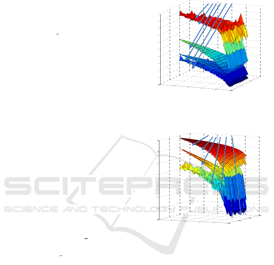
To demonstrate that ill-conditioning of the matrix
may really cause problems, a simple example is
demonstrated. Consider the sigmoid activation
functions with input weights and biases taken
randomly according to the uniform distribution in the
interval [-1,1], samples selected according to the
same distribution in the unit cube and calculate the
(
). The mean of condition coefficients
obtained in 20 experiments, for several numbers of
inputs is presented in fig. 1.
The number of hidden neurons was always smaller
than a half of a number of samples. The condition
number of
increases rapidly with a number of
neurons and samples. Performing any calculations
with the numbers as big as 10
14
in the matrix Λ
is
not reasonable.
As it is visible, the problem of ill-conditioning
escalates for small-dimensional modeling,
paradoxically. The regularization is not able to solve
this difficulty efficiently. To keep the condition
number in reasonable constraints
<10
must be
used, as it is presented in fig. 2. It is much bigger than
typically applied values
=50×ℎ.
3 ENHANCED VARIATION OF
ACTIVATION FUNCTIONS
The ELM is not able to learn the features from the
data, as a fully trained neural network does. The
randomly chosen weights happen to specify a linear
mapping to the space of neuron arguments. There-
fore the nonlinear mapping of the data into a feature
space should be able to extract the features sufficient
for predicting the target variable of a regression task.
It is not achieved at all times if the typical rules of
neuron construction (described in section 2) are
applied.
Figure 1: Logarithm of the condition number of
as a
function of batch size and the number of hidden neurons for
different number of inputs.
Figure 2: Logarithm of the condition number of
as a
function of batch size and the number of hidden neurons for
different number of inputs and the regularisation parameter
=10
.
For instance consider a case with 4 neurons, 2 inputs,
100 samples, weights and biases selection according
to the uniform distribution in [-1,1]. The mean
condition number of
in 2000 experiments is ∼
10
and the exemplary plots of activation functions
(from the last experiment) are presented in fig. 3.
It may be noticed that the activation functions are
almost linear and that the range of theirs outputs is
limited.
The importance of sufficient AFs variability was
noticed previously (Parviainen and Riihimäki, 2013),
(Kabziński, 2015). The challenge is to correct the
random mechanism of weights and biases creation to
increase variability without losing too much from the
simplicity of random selection.
0
100
200
300
0
20
40
60
80
100
2
4
6
8
10
12
14
16
18
20
22
No.of Samples
No of Inputs= , 1, 2, 5, 10, 20, 40
No. of Neuron
s
log10(mean(cond(H*H
T
)))
0
100
200
300
0
20
40
60
80
100
2
3
4
5
6
7
8
9
No.of Samples
No of Inputs= , 1, 2, 5, 10, 20, 40
No. of Neurons
log10(m ean( cond (H*H
T
)))
Extreme Learning Machine with Enhanced Variation of Activation Functions
79

Figure 3: Plots of exemplary sigmoid activation functions
obtained from a standard ELM.
For sigmoid AFs the following procedure may be
proposed:
The first step to enlarge the variation of a sigmoid
activation function is to increase the range of uniform
random selection of input weights. It must be suitably
fixed to guarantee that the sigmoid operation neither
remains linear nor too strongly saturates in the input
domain. Therefore the weights are selected from
uniform random distribution in the interval
[
−,
]
.
The values 5<<10 seems suitable.
The selected weights for the k-th neuron are divided
into positive and negative.
Next, the biases may be selected to ensure that the
range of a sigmoid function is sufficiently large. The
minimal value of the sigmoid function
ℎ
(
)
=
(
)
(13)
in the unit cube is achieved at the vertex selected
according to the following rules:
,
>0⇒
=0,
,
<0⇒
=1=1,…,,
(14)
and equals
ℎ
,
=
(
∑
,
:
,
)
, (15)
while the maximal value is achieved at the point given
by:
,
>0⇒
=1,
,
<0⇒
=0=1,…,
(16)
and equals
ℎ
,
=
(
∑
,
:
,
)
. (17)
Assuming that the minimal value of sigmoid AF
should be smaller than the given
, and the maximal
value should be bigger than
, 0<
<
<1
yields the range for the bias selection. It follows from
the inequalities
ℎ
,
<
,ℎ
,
>
, (18)
that the bias
should be selected on random,
uniformly from
∈[,], where
=−
∑
,
:
,
−
−1, (19)
=−
−1−
∑
,
:
,
. (20)
Of course, this approach does not guarantee that the
range of the AF will be
[
,
]
, as the parameters are
still random variables, but at least has chance to be.
A similar strategy may be applied for other
“projection based” AFs.
4 EFFECTIVENESS OF ELM
WITH ENHANCED VARIATION
OF ACTIVATION FUNCTIONS
To demonstrate the effectiveness of the proposed
method, consider a two-dimensional function
=sin(2
(
+
)
,
,
∈[0,1]. (21)
200 samples selected on random constitute the
training set, and 100 samples the testing sets. The
surface (21) was modeled by the standard ELM (S-
ELM), ELM with the enhanced variation of AFs (EV-
ELM) with parameters
=0.1,
=0.9, standard
ELM with regularization (R-ELM) and ELM with
regularization and the enhanced variation of AFs
(EV-R-ELM) with parameters =10
,
=
0.1,
=0.9.
In fig. 4,5 the modeling errors and the conditioning of
S-ELM and EV-ELM are compared. Application of
EV-ELM allows smaller modeling errors and far
better numerical properties of the obtained model.
The output weights are ~10
times smaller in EV-
ELM then in S-ELM.
The reason for this improvement is visible in fig. 6
where the plots of 4 AFs (selected from 60) are
presented. Fig. 6 and 3 demonstrate that in EV-ELM
AFs are nonlinear and cover wider subinterval in
[0,1], however not all of them vary from
to
.
The advantage of EV-ELM is even more obvious if it
is applied together with the regularization. Fig. 7, 8
demonstrate the comparison between R-ELM and
0
0.5
1
0
0.5
1
0.4
0.5
0.6
0.7
0.8
x
y
0
0.5
1
0
0.5
1
0.4
0.5
0.6
0.7
0.8
x
y
0
0.5
1
0
0.5
1
0.7
0.8
0.9
x
y
0
0.5
1
0
0.5
1
0.55
0.6
0.65
x
y
NCTA 2016 - 8th International Conference on Neural Computation Theory and Applications
80
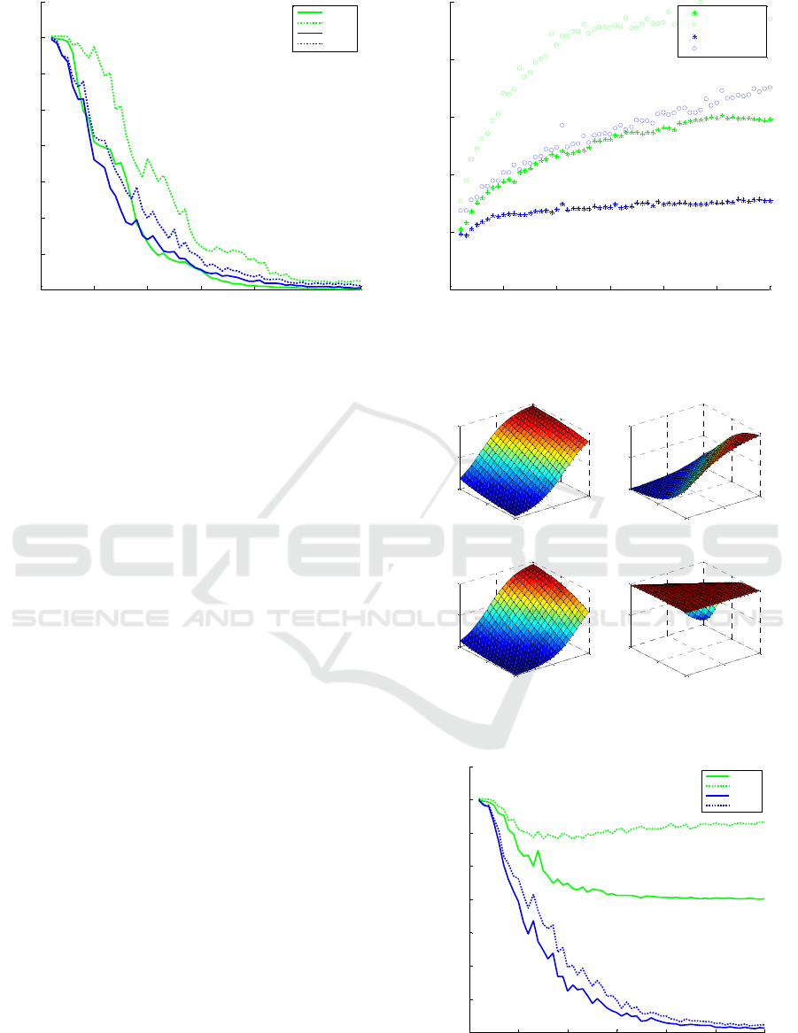
Figure 4: Testing (dotted) and training (solid) errors for S-
ELM (brighter - green) and EV-ELM (darker – blue).
EV-R-ELM. The regularization alone is able to keep
the output weights on a moderate level, but the
modeling becomes unacceptably inaccurate. The EV-
R-ELM improves the modeling accuracy and the
conditioning together. Similar experiments were
conducted for different modeling problems: with the
training output corrupted by noise, with multiple
inputs, with numerous extrema, and always the
conclusions were similar.
5 CONCLUSIONS
The main aim of this paper was to stress the fact that
the sufficient variability of AFs is important for an
ELM model accuracy and applicability. A slight
modification of the standard ELM procedure is
proposed, which allows enhancing the variance of
each AF, without losing too much from the simplicity
of random selection of parameters.
First, it is proposed to change the parameter of the
random distribution of the input weights, next to
modify the random distribution for the basses, taken
already established weights into account. The
proposed modification does not increase the
computational complexity of an ELM training
significantly – only two simple calculations for each
bias are added. Enhancing the variation of AFs results
in reduced output weights norm, better numerical
conditioning of the output weights calculation,
smaller errors for the same number of the hidden
neurons. The proposed approach works efficiently
together with the Tikhonov regularization applied in
ELM.
Figure 5: Logarithm of the norm of the output weights
(stars) and ((
) (circles) for S-ELM (brighter
- green) and EV-ELM (darker – blue).
Figure 6: Selected AFs (4 from 60) from the EV-ELM
model.
Figure 7: Testing (dotted) and training (solid) errors for R-
ELM (brighter - green) and EV-R-ELM (darker – blue).
0 10 20 30 40 50 60
0
0.1
0.2
0.3
0.4
0.5
0.6
0.7
0.8
No of hidden neurons
ELM errors
train err.
test er r.
train err.
test er r.
0 10 20 30 40 50 60
-5
0
5
10
15
20
No of hidden neurons
log(norm(OW )
log( c ond( H*H
T
)
log(norm(OW )
log( c ond( H*H
T
)
0
0.5
1
0
0.5
1
0
0.5
1
x
1
X
2
0
0.5
1
0
0.5
1
0
0.5
1
x
1
X
2
0
0.5
1
0
0.5
1
0
0.5
1
x
1
X
2
0
0.5
1
0
0.5
1
0
0.5
1
x
1
X
2
0 10 20 30 40 50 60
0
0.1
0.2
0.3
0.4
0.5
0.6
0.7
0.8
No of hidden neurons
ELM errors
train err .
test er r.
train err .
test er r.
Extreme Learning Machine with Enhanced Variation of Activation Functions
81
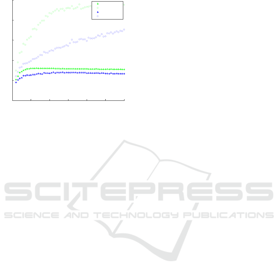
Figure 8: Logarithm of the norm of the output weights
(stars) and ((
) (circles) for R-ELM (brighter
- green) and EV-R-ELM (darker – blue).
REFERENCES
Akusok, A., Bjork, K. M., Miche, Y., and Lendasse, A.
(2015). High-Performance Extreme Learning Machi-
nes: A Complete Toolbox for Big Data Applications.
IEEE Access, 3, 1011–1025. http://doi.org/10.1109/
ACCESS.2015.2450498
Chen, Z. X., Zhu, H. Y., and Wang, Y. G. (2013). A
modified extreme learning machine with sigmoidal
activation functions. Neural Computing and
Applications, 22(3-4), 541–550. http://doi.org/10.1007/
s00521-012-0860-2
Feng, G., Lan, Y., Zhang, X., and Qian, Z. (2015). Dynamic
adjustment of hidden node parameters for extreme
learning machine. IEEE Transactions on Cybernetics,
45(2), 279–288. http://doi.org/10.1109/TCYB.2014.23
25594
Guang-Bin Huang, and Chee-Kheong Siew. (2004).
Extreme learning machine: RBF network case. In
ICARCV 2004 8th Control, Automation, Robotics and
Vision Conference, 2004. (Vol. 2, pp. 1029–1036).
IEEE. http://doi.org/10.1109/ICARCV.2004.1468985
Huang, G., Huang, G. Bin, Song, S., and You, K. (2015).
Trends in extreme learning machines: A review. Neural
Networks, 61, 32–48. http://doi.org/10.1016/j.neunet.
2014.10.001
Kabziński, J. (2015). Is Extreme Learning Machine
Effective for Multisource Friction Modeling? (in
Artificial Intelligence Applications and Innovations,
Springer pp. 318–333). http://doi.org/10.1007/978-3-
319-23868-5_23
Lin, S., Liu, X., Fang, J., and Xu, Z. (2015). Is extreme
learning machine feasible? A theoretical assessment
(Part II). IEEE Transactions on Neural Networks and
Learning Systems, 26(1), 21–34. http://doi.org/10.
1109/TNNLS.2014.2336665
Liu, X., Lin, S., Fang, J., and Xu, Z. (2015). Is extreme
learning machine feasible? A theoretical assessment
(Part I). IEEE Transactions on Neural Networks and
Learning Systems, 26(1), 7–20. http://doi.org/10.1109/
TNNLS.2014.2335212
Miche, Y., Sorjamaa, A., Bas, P., Simula, O., Jutten, C., and
Lendasse, A. (2010). OP-ELM: Optimally pruned
extreme learning machine. IEEE Transactions on
Neural Networks, 21(1), 158–162. http://doi.org/10.
1109/TNN.2009.2036259
Miche, Y., van Heeswijk, M., Bas, P., Simula, O., and
Lendasse, A. (2011). TROP-ELM: A double-regulari-
zed ELM using LARS and Tikhonov regularization.
Neurocomputing, 74(16), 2413–2421. http://doi.org/
10.1016/j.neucom.2010.12.042
Parviainen, E., and Riihimäki, J. (2013). A connection
between extreme learning machine and neural network
kernel. In Communications in Computer and
Information Science (Vol. 272 CCIS, pp. 122–135).
0 10 20 30 40 50 60
-5
0
5
10
15
20
No of hidden neurons
log(norm(OW)
log(c ond( H*H
T
)
log(norm(OW)
log(c ond( H*H
T
)
NCTA 2016 - 8th International Conference on Neural Computation Theory and Applications
82
