Exploring the Neurosolver in Playing Adversarial Games

Andrzej Bieszczad

Computer Science, California State University Channel Islands, One University Drive, Camarillo, CA 93012, U.S.A.

Keywords: Neural Network, Neurosolver, General Problem Solving, State Spaces, Search, Adversarial Search, Temporal

Learning, Neural Modeling.

Abstract: In the past, the Neurosolver, a neuromorphic planner and a general problem solver, was used in several

exploratory applications, such as Blocks World and Towers of Hanoi puzzles, that in which we investigated

its problem solving capabilities. In all of them, there was only one agent that had a single point of view focus:

how to solve a posed problem by generating a sequence of actions to get the system from its current state to

some goal state. In this paper, we report on our experiments with exploring the Neurosolver’s capabilities to

deal with more sophisticated challenges in solving problems. For that purpose, we employed the Neurosolver

as a driver for adversary games. In that kind of environment, the Neurosolver cannot just generate a plan and

then follow it through. Instead, the plan has to be revised dynamically step by step in response to the other

actors following their own plans realizing adversarial points of view. We conclude that while the Neurosolver

can learn to play an adversarial game, to play it well it would need a good teacher.

1 INTRODUCTION

The goal of the research that led to the original

introduction of Neurosolver, as reported in

(Bieszczad et al., 1998), was to design a

neuromorphic device that would be able to solve

problems in the framework of the state space

paradigm. Fundamentally, in this paradigm, a

question is asked how to navigate a system through

its state space so it transitions from the current state

into some desired goal state. The states of a system

are expressed as points in an n-dimensional space.

Trajectories in such spaces formed by state transitions

represent behavioral patterns of the system. A

problem is presented in this paradigm as a pair of two

states: the current state and the desired, or goal, state.

A solution to the problem is a trajectory between the

two states in the state space.

The Neurosolver can solve such problems by first

building a behavioral model of the system and then

by traversing the recorded trajectories during both

searches and resolutions as will be described in the

next section.

In this paper, we report on our explorations of the

capabilities of the Neurosolver to construct a

behavioral model for carrying out more complex

tasks. For that purpose, we employed it as a controller

for playing an adversarial game. Specifically, we

used a variety of versions of the Neurosolver and

training techniques to construct automatically a driver

for the computer player in the game of TicTacToe.

The Neurosolver has proven itself as a reliable

problem solver finding trajectories in problem spaces

of several problems between the current system state

and the desired goal state (Bieszczad, 2006, 2007,

2011, 2015). In the application reported in here, the

Neurosolver confirms that it is a reliable tool for

producing sequences between two configurations of

the TicTacToe board. However, an adversarial game

is an interactive activity rather than a plan prepared a

priori and then followed through. Simply, adversaries

do not follow the same plan (and especially the plans

of their opponents!), so the Neurosolver must

recalculate the plan after each adversarial move. That

requires more time, but again it’s something that the

Neurosolver can handle well. Unfortunately, that is

not all; the rules of the game must be followed and

not all configurations are allowed to be successors of

a given move, even though they might be minimizing

the path to a goal (i.e., one of the winning game

configurations). That is a particularly unpleasant

challenge for automated training that uses randomly

generated games for training, since even if the game

ends with a winning configuration, it is difficult to

evaluate the player’s quality reliably.

The original research on Neurosolver modeling

was inspired by Burnod’s monograph on the

workings of the human brain (Burnod, 1988). The

Bieszczad, A.

Exploring the Neurosolver in Playing Adversarial Games.

DOI: 10.5220/0006070800830090

In Proceedings of the 8th International Joint Conference on Computational Intelligence (IJCCI 2016) - Volume 3: NCTA, pages 83-90

ISBN: 978-989-758-201-1

class of systems that employ state spaces to present

and solve problems has its roots in the early stages of

AI research that derived many ideas from the studies

of human information processing; among them on

General Problem Solver (GPS) (Newell and Simon,

1963). This pioneering work led to very interesting

problem solving (e.g. SOAR (Laird, Newell, and

Rosenbloom, 1987)) and planning systems (e.g.

STRIPS (Nillson, 1980).

The Neurosolver employs activity spreading

techniques that have their root in early work on

semantic networks (e.g., (Collins and Loftus, 1975)

and (Anderson, 1983)).

The Neurosolver is a network of interconnected

nodes. Each node is associated with a state in a

problem space. In the case of the TicTacToe game, a

state is associated with a single configuration of the

board. In its original application, the Neurosolver is

presented with a problem by two signals: the goal

associated with the desired state and the sensory

signal associated with the current state. In the context

of the TicTacToe game, the current state is the initial

broad configuration (i.e., an empty board), and the

desired state is one of the winning board

configurations. A sequence of firing nodes that the

Neurosolver generates represents a trajectory in the

state space. Therefore, a solution to the given problem

is a succession of firing nodes starting with the node

corresponding to the current state of the system, and

ending with the node corresponding to the desired

state of the system. In case of the TicTacToe game, a

sequence represents a winning game.

The node used in the Neurosolver is based on a

biological cortical column (references to the relevant

neurobiological literature can be found in (Bieszczad,

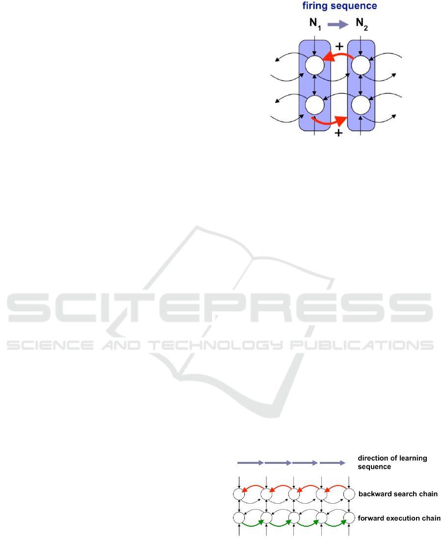
1998)). It consists of two divisions: the upper and the

lower, as illustrated in Figure 1. The upper division is

a unit integrating internal signals from other upper

divisions and from the control center providing the

limbic input (i.e., a goal or — using more psycholo-

gycal terms — a drive or desire). The activity of the

upper division is transmitted to the lower division

where it is subsequently integrated with signals from

other lower divisions and the thalamic (i.e., sensory)

input. The upper divisions constitute a network of

units that propagate search activity from the goal,

while the lower divisions constitute a network of

threshold units that integrate search and sensory

signals, and subsequently generate sequences of

firing nodes. A sequence of outputs of the lower

divisions of the network constitutes the output of the

whole node; a response of the network to the input

stimuli.

Figure 1: Neurosolver learning rule.

In the original Neurosolver, the strength of all

inter-nodal connections is computed as a function of

two probabilities: the probability that a firing source

node will generate an action potential in this

particular connection, and the probability that the

target node will fire upon receiving an action

potential from the connection.

An alternate implementation follows the Hebbian

approach that increments the strength of the

connection that carried the action potential that cause

the recipient to fire. In this approach, a certain small

value is added to the weight of a connection on each

successful pairing. To keep the values under control

all weights of afferent and efferent connections may

be normalized so their sum does not exceed 1. This

model approximates well the statistical model

described in the previous paragraph.

One other option for training is making all

weights the same (for example, equal to 1);

alternately, the weights may be ignored completely to

improve efficiency. In this approach, multiple

presentations of data do not affect the model. In such

implementation, the system produces optimized

(shortest) solution paths that are independent of the

frequency of sample presentations.

Figure 2: Learning state space trajectories through bi-

directional traces between nodes corresponding to

transitional states of the system.

TicTacToe (also know as “noughts and crosses”

or “Xs and Os”) is a very popular game that is very

NCTA 2016 - 8th International Conference on Neural Computation Theory and Applications

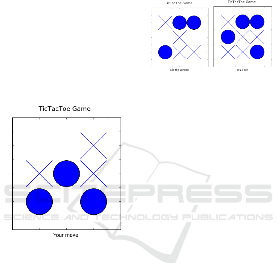
simple in its most fundamental form using a board of

9 squares that can be either empty or hold one of the

the two player symbols: a cross or a circle (or some

other markers) as shown in Figure 3.

Each of the two players is assigned one of the two

symbols: a cross (‘X’) or a circle (‘O’). The game

proceeds by placing players symbols on the still

empty board squares. The objective of the game is to

align 3 same symbols in a vertical, horizontal, or

diagonal line.

There are numerous variations of the game; e.g.,

larger boards can be used, including a border-less

version. As well, the number of symbols in a winning

arrangement may vary.

Figure 3. A TicTacToe board used in the experiments. The

board shows the configuration encoded as ‘001121202’ in

the implementation.

TicTacToe has been used extensively in research

on Artificial Intelligence (e.g., Russell et al., 2010),

because its problem space is manageable, so even an

exhaustive search can be used on today’s computers

in case of its simpler versions. For example, the

number of states in a 3-by-3 version used in the work

reported here is 3

=19,683 and the number of possible

games is 9!=362,880. Each game is a sequence of

moves from the the board with all empty squares to

one of the final configurations representing either a

win for ‘X’, or a win for ‘O’, or a tie. There are two

final configurations shown in Figure 4. Usually, the

problem space is considerably reduced by

preprocessing that reflects a number of observations

such as board symmetry, rotation, and player

symmetry.

Figure 4. Two board configurations showing a win for

crosses encoded as ‘122010211’ (left side) and a tie

encoded as ‘122211112’.

2 IMPLEMENTATION

2.1 Models

In this implementation, each state of the puzzle is

represented internally as as a 9-element string of

characters ‘0’, ‘1’, and ‘2’ representing the

configuration of the board. The string is constructed

by concatenating 3-element strings representing each

of the rows in the board. ’0’ represents and empty

square, ‘1’ - an ‘X’, and ‘2’ - an ‘O’. Using numbers

rather than letters helps internally as the game is

implemented in Python using the NumPy library, and

it’s easy to move a configuration to a NumPy array

for some flexible operations provided by that library.

There are some examples of the configuration

representation shown in Figures 4 and 5.

The Neurosolver consists of a collection of nodes

representing the configurations (states) of the board.

Each node has two dictionaries that represent efferent

and afferent connections with keys being string

representations of neighboring configurations (states)

and values representing the corresponding weights. A

node can be activated up to a certain platform

maximum that can be adjusted to control the time that

the Neurosolver is given to perform computations.

There are two activity thresholds that control activity

propagation for searching and for following solutions

as explained shortly.

2.2 The Neurosolver Operation

The Neurosolver requires three main stages to solve a

problem: training, searching, and solving.

These stages can be interwound in online learning

mode. In the offline learning mode the first stage is

separated from the two others.

Exploring the Neurosolver in Playing Adversarial Games

2.2.1 Training

As training sample games are presented to the

Neurosolver, nodes and connections are added to the

model. A node is added to the Neurosolver when a

corresponding configuration (state) is present as one

element of a training sample. Consecutive pairs of

board configurations represent transitions between

configurations; they constitute game moves. During

training, the Neurosolver is presented with all moves

in each training sample game. If not yet in the model,

a node representing a configuration is added when the

configuration represents the first element of the

sample pair, or when it is presented as the target of

the transition. Learning always affects two nodes: a

‘from’ node and a ‘to’ node. The dictionaries holding

references to nodes representing forward and

backward neighbors (successors and predecessors) in

the training sample are constructed in the process. In

the Hebbian model, the weights are adjusted

accordingly by incrementing them by a certain value

and normalizing. In the model with fixed cone-ctions,

just a fact of being a neighbor matters, so the weights

in that case are ignored and not adjusted.

The implementation includes offline and online

modes. In the online mode both a command line and

GUI interfaces were implemented. Figures 4 and 5

show the GUI interface. However, training - although

preferable due to the human involvement in

evaluating the quality of the training samples as

explained later - using such manual approach is very

time consuming. To make the process fast, a game

generator has been implemented. The generator

ensures that a valid game is generated by randomly

generating the next valid board configuration and

testing whether the most recently generated

configuration is one of the final states. If the final

state in the generated game is the winner or a tie, the

whole game is presented as a learning sample to the

Neurosolver. With the spirit of learning from

somebody else’s experience, a game won by the

adversary (the human player) the game is transitioned

to a form that represents exactly same sequence of

moves but with the computer as the winner and also

used as a training sample. The process merely substi-

tutes all ‘1s’ to ‘2s’ (i.e., ’Xs’ to ‘Os’) and vice versa.

The ties were added to the training because they

evidently improved the capabilities of the model as

shown in the section analyzing the experimental data.

2.2.2 Searching

After the training is complete, the Neurosolver will

have built a connection map between numerous states

of the problem domain. The next step is to activate

the node representing the goal state and allow the

propagation process to spread this search activity

along the connection paths in the direction that is

reverse to the flows of sample games used in training.

If there were only one game learned, then the flow

would be from the last configuration to the first.

There are however many training samples used in

training, so the activity spreads out as a search tree

looking for the node representing the starting state.

The extent of the search tree is controlled by imposing

a search threshold; a node that is a leaf in the search

tree is allowed to propagate its activity further only if

its activity exceeds the value of the search threshold.

The starting node is activated in preparation for

incoming search activity flow, so when that activity

reaches it the node may fire if its activity exceeds the

firing threshold. At that moment, the next stage of the

Neurosolver operation, solving, will start. That

process is explained in the next section.

A TicTacToe Game data set from UCI repository

was used as the basis of a data set to select the goals.

The UCI set only shows negative and positive

outcomes for ‘Xs’. Using the UCI set, a data set of all

non-loosing states was produced. Each game in the

new set was labeled with ‘1’ for ‘X’ winners, ‘2’ for

‘O’ winners, and with ‘3’ for ties. The new set was

used for two types of training sessions: one with ties

included and another one with ties excluded. The

section analyzing the results illustrates the impact of

using ties in the learning process.

2.2.3 Solving

The last stage of the Neurosolver is to actually use all

of the information collected thus far, and to generate

an actual solution from the given current state to the

specified goal state. Since all the nodes in the search

tree are activated, we may consider them in

anticipating state for the firing sequence. Therefore,

when the firing node projects its activity weighted by

the strength of the forward connections, the neighbor

that has the highest anticipatory activity will fir next,

That node is added to the solution, and then process

repeats itself until the goal state is reached. When that

happens, the solution to the problem has been

produced.

However, in contrast to the earlier experimental

application of the Neurosolver, in adversarial games

there are no single “solutions” that can be generated

once up front and then used as a recipe to “solve the

problem”. Hence, firstly there are many possible

goals, so all of them get activated to start the search.

In this way, the propagation process constructs

multiple search trees. Since they span the same

NCTA 2016 - 8th International Conference on Neural Computation Theory and Applications

network, the trees are not independent, so the activity

from one goal affects trees rooted in other goal states.

Secondly, the need arises to generate a single “next

state” rather than a complete solution. Accordingly,

the operation of the Neurosolver has been augmented

by facility to produce one configuration rather than

the whole sequence to one of the goal states. The

latter would be rather unusable, since the adversaries

usually do not follow each other advice.

The next move can be suggested quickly in the

model using Hebbian learning by following the

strongest connection from the node corresponding to

the current state. However, that approach just follows

the frequency of training moves (state transitions) and

is unreliable with automated training that uses

random training samples. A ore reliable approach is

to use the same activity propagation process as

described, however collecting only the first transition

rather than the complete solution. That process must

be repeated for every game turn of the computer

player. Hence, there are numerous solving processes

involved in playing a single game.

In the model with the fixed weights, activity spre-

ading is the only way to find suggested moves, since

there is no probabilistic model to take advantage of.

3 EXPERIMENTS

Measuring the quality of the model is a challenge due

to the difficulty is evaluating quantitatively the

quality of moves. A computer player controlled by the

Neurosolver can be evaluated qualitatively by an

adversary human player, but that is limited and

somewhat subjective.

To get some quantitative measure of the

Neurosolver capabilities, we used the data set from

UCI to create a test set that includes all possible

problems (games; i.e., sequences of moves) with the

original board configuration with all squares empty as

the current (start) state to a state representing every

possible winning (for a selected player; ‘X’ or ‘O’)

board configuration. We conducted several

experiments trying to select the best training strategy.

The following sections describe the results.

In each of the experiments, we created five

models of the Neurosolver-based TicTacToe

controller each trained with progressively increasing

number of sample games. Each game was generated

randomly by generating valid moves and testing for

the terminal state at every step. We experimented

with varied number of presentations of each game,

but ultimately decided that it’s better to spend the

same time on generating more variety of games rather

than reinforcing ones that were already presented.

Therefore, each game was presented only once when

generated. We allowed for repeats if the random

process happened to produce a game more than once.

The probability of that is not very high taking into

account the number of possible games.

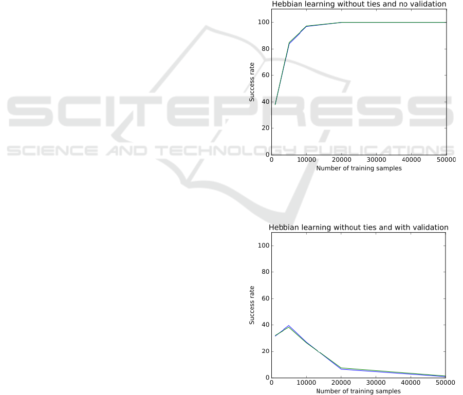
3.1 Hebbian Learning with No Ties

and No Move Validation

In this experiments, we wanted to know if the

Neurosolver performs as in the past on the problems

that are solved by producing state transition paths

between the start state and the goal state in the state

space. In this session, we used only winning states as

the goal states, and we did not validate the generated

moves. We just wanted to confirm that the

Figure 5: Success rate of the model built using the Hebbian

learning with ties excluded and the validation of moves

turned off.

Figure 6: Success rate of the model built using the Hebbian

learning with ties excluded and the validation of moves

turned on.

Exploring the Neurosolver in Playing Adversarial Games

Neurosolver behaves in the same way as in the past

applications.

It appears that the resulting model reliably

produces paths between the starting board

configurations and every winning terminal state as

shown in Figure 5. With 1000 training samples the

success rate measured as the percentage of successful

attempts to find a path between the start and the goal

is around 40%. With 10000 sample, the performance

starts to approach 100%, and with 20000 samples and

more the system is nearly perfect.

3.2 Hebbian Learning with No Ties

and with Move Validation

The results from the first experiment session were

very promising. To validate the games we built a

move validator that ensures that every move

generated by the Neurosolver is actually valid

according to the TicTacToe rules. In the following

session, we validated every game (i.e., every solution

path) generated by the Neurosolver. If a game did not

validate (i.e., if it included at least one invalid move),

the attempt was marked as a failure.

The results shown in Figure 6 illustrate the

problem with applying the Neurosolver in a context

in which not only the path, and even the path length,

matter, but also the “quality” of the solution that must

adhere to some externally-imposted standards. While

initially the success rate is similar to the previous

model, increasing the number of training samples

lowers the success rate dramatically. With 20000 or

more training samples, the model failed for most

posed problems.

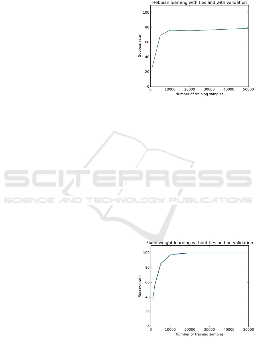
3.3 Hebbian Learning with Ties and

with Move Validation

The results from the second experiment session were

not good to say the least. When playing against the

computer, we noticed that it was better being

offensive than defensive, so we decided to also use

the tying games in the training to teach the model

some defensive strategies; e.g., to block adversarial

moves. It was quite a surprise to see that including

ties actually improved the quality of solutions quite

dramatically.

As shown in Figure 7, the model built with a data

set that included the tying games brought the success

rate close to 80% already for 10000 training samples.

The rate changed minimally with increased number

of training samples. That is an important observation,

since increasing the number of training samples. The

rate changed minimally with increased number

Figure 7: Success rate of the model built using the Hebbian

learning with ties included and the validation of moves

turned on.

of training samples. That is an important observation,

since increasing the number of training samples

increases dramatically the time necessary for building

the model, and also - albeit not dramatically - the time

for producing a solution. The latter might be a bit

surprising, but the reason for that is that more samples

lead to larger search activity trees.

3.4 Fixed-weight Learning with No

Ties and No Move Validation

As we explained earlier, the Neurosolver models with

fixed connection weights are good optimizers

producing shortest paths. Since the drive to move to

a goal might be a good capability for suggesting

better, more aggressive moves, we also built two

models to test this hypothesis.

Figure 8. Success rate of the model built using the fixed-

weight learning with ties excluded and the validation of

moves turned off.

NCTA 2016 - 8th International Conference on Neural Computation Theory and Applications

The first model was built with games ending in

tying configurations excluded and with no validation

of moves. As shown in Figure 8, this model

performed as well as the model crated using the

Hebbian learning. With 10000 training the success

rate approached 100%. We did not compare the

lengths of the produced games (i.e., the lengths of the

solution paths), but one could suspect that they would

tend to be shorter in this model.

3.5 Fixed-Weight Learning with No

Ties and with Move Validation

As with the models built with the Hebbian approach,

we wanted to evaluate the quality of the solutions, so

we used exactly same method that validated all moves

in each produced game.

As shown in Figure 9, the quality of the games is

as bad, and it goes down with the increasing number

of training samples.

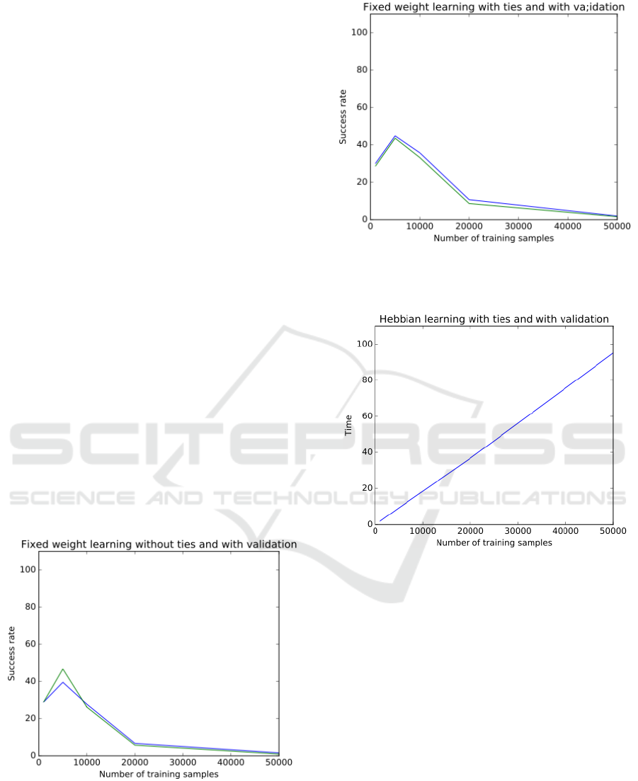
3.6 Fixed-Weight Learning with Ties

and with Move Validation

To next question was whether including the tying

games in training would also improve the ability of

the fixed-weight model to generate quality games.

Unfortunately, as shown in Figure 10, the trick

that was so useful in the Hebbian model did not work

here. The success rate of the model built with the

tying games included in training is as bad as of the

model built without ties included.

Figure 9: Success rate of the model built using the fixed-

weight learning with ties excluded and the validation of

moves turned on.

Figure 10: Success rate of the model built using the fixed-

weight learning with ties included and the validation of

moves turned on.

Figure 11: Sample time necessary to construct the model

using the Hebbian learning.

3.7 Time to Build Models

The time necessary to build the models depends on

the computing platform, of course. Nevertheless,

looking at the trends might be informative.

Figure 11, includes a graph that shows how the

time required to train a Hebbian model (with ties

excluded, to be precise) increases as a function of the

training samples. As shown, the dependency is linear.

It is worth noting, that evidently that is the trend as in

one session the training time rose to close to 600

seconds for a training sample of 300000 games. That

would be an approximate value if the graph from

Figure 11 was used for extrapolation.

Exploring the Neurosolver in Playing Adversarial Games

3.8 Qualitative Evaluation

We played with the Neurosolver-driven computer

player numerous games. Although the current best

model (see Figure 7) shows some signs of decent

playing skills, it is far from satisfactory. The model

seems to be superior in offensive strategies, but

evidently does not acquire skills necessary to prevent

some obvious moves, like blocking placing the third,

winning, adversarial symbol in a line.

4 CONCLUSIONS

In the line of experiments reported in this paper, we

showed that the Neurosolver can find paths between

the starting TicTacToe board configuration and any

winning state with very high success just after

sampling 10000 out of 9! possible games. However,

finding a path is not sufficient in the application of

the Neurosolver as a controller for driving a computer

player in an adversarial game. In this application, the

quality of the game measured by its validity as well

as an ability to interactively produce “good” moves is

of paramount importance. The strategies used for

training the Neurosolver yielded only moderate

success. The main reason for that is the automated

process that can validate games, but cannot evaluate

the quality of individual moves.

The Neurosolver is a device that learns by being

told, so employing either a skillful human or

computer player, or a data set of “good” games, seems

to be necessary to acquire good playing skills. For

example, the common heuristic utility function for

TicTacToe configurations could be used to generate

more promising moves. The point of our experiments,

however, was to see if such heuristics can be

developed automatically. The current answer to that

question is a sound ‘no’.

Our next goal is to identify states from the raw

images of the TicTacToe board and to acquire the

behavior without explicit representation of the state

space. We hope to build a model from scratch by

putting together a deep learning front end (e.g.,

convolution networks (Lawrence at al., 1998)) with

the Neurosolver back end.

REFERENCES

Anderson, J. R., 1983. A spreading activation theory of

memory. In Journal of Verbal Learning and Verbal

Behavior, 22, 261-295.

Bieszczad, A. and Pagurek, B., 1998. Neurosolver:

Neuromorphic General Problem Solver. In Information

Sciences: An International Journal 105, pp. 239-277,

Elsevier North-Holland, New York, NY.

Bieszczad, A. and Bieszczad, K., (2006). Contextual

Learning in Neurosolver. In Lecture Notes in Computer

Science: Artificial Neural Networks, Springer-Verlag,

Berlin, 2006, pp. 474-484.

Bieszczad, A. and Bieszczad, K., (2007) Running Rats with

Neurosolver-based Brains in Mazes. In Journal of

Information Technology and Intelligent Computing,

Vol. 1 No. 3.

Bieszczad A., (2011). Predicting NN5 Time Series with

Neurosolver. In Computational Intelligence: Revised

and Selected Papers of the International Joint

Conference IJCCI 2009 (Studies in Computational

Intelligence). Berlin Heidelberg: Springer-Verlag, pp.

277-288.

Bieszczad, A., and Kuchar, S., (2015) The Neurosolver

Learns to Solve Towers of Hanoi Puzzles. In

Proceedings of 7th International Joint Conference on

Computational Intelligence (IJCCI 2015), Lisbon,

Portugal.

Burnod, Y., 1988. An Adaptive Neural Network: The

Cerebral Cortex, Paris, France: Masson.

Collins, Allan M.; Loftus, Elizabeth F., 1975. A Spreading-

Activation Theory of Semantic Processing. In

Psychological Review. Vol 82(6) 407-428.

Laird, J. E., Newell, A. and Rosenbloom, P. S., 1987.

SOAR: An architecture for General Intelligence. In

Artificial Intelligence, 33: 1--64.

Lawrence, S., et al., 1998. Face Recognition: A

Convolutional Neural-Network Approach. In IEEE

Transactions on Neural Networks, Vol 8(1), pp.98-113.

Newell, A. and Simon, H. A., 1963. GPS: A program that

simulates human thought. In Feigenbaum, E. A. and

Feldman, J. (Eds.), Computer and Thought. New York,

NJ: McGrawHill.

Nillson, N. J., 1980. Principles of Artificial Intelligence,

Palo Alto, CA: Tioga Publishing Company.

Russell, S. J., Norvig, P., 2010. Artificial Intelligence: A

Modern Approach (3rd ed.), Pearson.

Stewart, B. M. and Frame, J. S., 1941. Solution to Advanced

Problem 3819. In The American Mathematical

Monthly Vol. 48, No. 3 (Mar., 1941), pp. 216-219

NCTA 2016 - 8th International Conference on Neural Computation Theory and Applications