Road Cycling Climbs Made Speedier by Personalized Pacing Strategies
Stefan Wolf
1
, Raphael Bertschinger
2
and Dietmar Saupe
1
1
Department of Computer and Information Science, University of Konstanz, Konstanz, Germany
2
Department of Sports Science, University of Konstanz, Konstanz, Germany
Keywords:
Optimal Strategies, Critical Power, Road Cycling, Optimal Feedback.
Abstract:
Lately, modeling and optimizing endurance performance has become popular. Optimal strategies have been
calculated for running as well as for cycling. Since most of these studies are of theoretical nature, we per-
formed a series of experiments to determine whether race performance can actually be improved using math-
ematical optimization in a realistic scenario. The optimal strategy was based on the equations of motion for
cycling and an individual critical power model for each rider. Constant visual feedback based on the calculated
strategy was given to the rider while performing a real world climb on a bike simulator in the laboratory. The
aim of this study was to determine whether these strategies are feasible and effective. The results showed that
feedback in general and the optimal strategy feedback in particular led to a significant improvement. The total
race times decreased between 0.8% and 3.2% employing optimal strategy feedback compared to self paced
rides.
1 INTRODUCTION
What makes a winner in endurance races like a Tour
de France stage? Besides pre-race preparations, the
strategy during the race has a major influence on vic-
tory or defeat. During recent years, optimizing pacing
strategies based on mathematical models has become
more and more popular. Mainly running and cycling
individual time trials have been investigated.
First results for cycling were gathered by Gor-
don (2005). The 3-parameter critical power model
of Morton (1996) and a simple mechanical model
which includes air resistance, friction and gravitation
were used to analytically calculate strategies on sim-
ple, piecewise constant courses.
An extension of this work has been provided by
Dahmen et al. (2012). The more realistic mechanical
model of Martin et al. (1998), which also includes in-
ertia and bearing friction as well as slope profiles of
real world courses has been used. Due to the higher
complexity of the optimization problem, numerical
methods were applied.
Since then several studies have been published
that apply more sophisticated physiological mod-
els. For example, Sundstr
¨
om et al. (2014) compared
strategies with the traditional critical power model to
a more versatile 3-component model which was intro-
duced by Morton (1986).
All of the current studies in this field are mainly
of theoretical nature and it still remains to be shown
whether one can improve realistic rides using opti-
mized strategies. For this purpose, we present an ex-
periment where a mathematically calculated, optimal
strategy has been used to provide visual feedback dur-
ing a simulated ride on a real world course in the lab-
oratory.
We provide an experimental setting to answer
whether the calculated optimal strategies are feasible
i.e. the riders are able to follow the strategy until the
end. Moreover, we determined the resulting improve-
ment in performance. This study presents the under-
lying mathematical models, the parameter estimation
process and the results.
2 METHODS
2.1 Experimental Setup
Six healthy male subjects (mean standard deviation;
age = 27.7 ± 4.2 years; height = 182.6 ± 5.3 cm;
weight = 76.3 ± 5.3 kg) participated in the study af-
ter giving informed consent. Aerobic capacity was
heterogeneous throughout the group of subjects, indi-
cated by the power to weight ratio at the blood lactate
threshold (Table 1). Subjects were asked to refrain
Wolf, S., Bertschinger, R. and Saupe, D.
Road Cycling Climbs Made Speedier by Personalized Pacing Strategies.
DOI: 10.5220/0006080001090114
In Proceedings of the 4th International Congress on Sport Sciences Research and Technology Support (icSPORTS 2016), pages 109-114
ISBN: 978-989-758-205-9
Copyright
c
 2016 by SCITEPRESS – Science and Technology Publications, Lda. All rights reserved
109

from caffeine and alcohol at least one night and from
intense physical activity at least two days prior the ex-
periment.
All tests were performed on a bike simulator based
on a Cyclus2 brake (RBM elektronik-automation
GmbH, Germany) and a customized simulator soft-
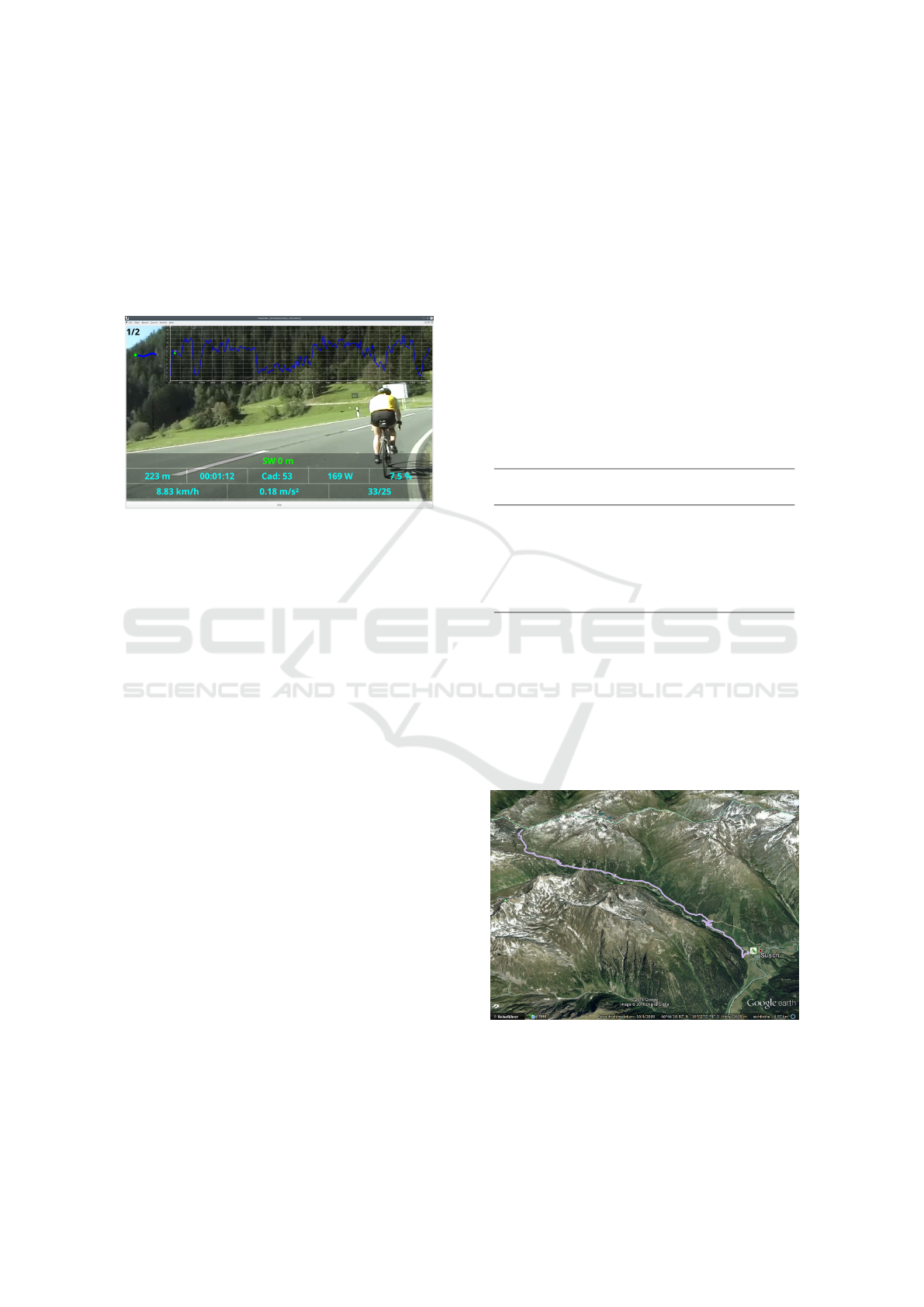
ware (Dahmen et al., 2011). Figure 1 shows the vi-
sual interface of the simulator which is projected on
the wall in front of the rider.
Figure 1: Visual interface of the simulator. The top graph
shows the slope profile and the position on the course. In the
background a video of the track is played which is synchro-
nized to the simulated speed. On the bottom current status
information like traveled distance, speed or power output is
shown. Best viewed electronically.
The experiment incorporated five tests with rest
periods of one week between each test. At first, each
subject performed an incremental step test to exhaus-
tion starting at 100 W with increments of 20W every
3 minutes to obtain an estimate of his anaerobic lac-
tate threshold (AT). The other tests were simulated
rides on a real course, namely the eastern climb of
the Fl
¨
uela Pass in Switzerland. More details about
the course are provided below.
The first simulation ride (I) was for familiariza-
tion purposes. In order to obtain a suitable bench-
mark, subjects were advised to ride close to their AT
but were free in the selection of their power output. In
the second ride (II) subjects rode with their own pac-
ing strategy. In rides I and II subjects were instructed
to perform with maximal effort.
The third ride (III) was performed with an optimal
strategy feedback and the fourth ride (IV) with a val-
idation strategy feedback. The optimal strategy was
obtained by solving the optimal control problem de-
scribed below. Whereas the energy expenditure in the
optimal strategy was similar to rides I and II, the race
time was shorter than that achieved in those rides.
The validation strategy was determined by adding
a constant power offset to the riders’ own strategy
of ride II in order to achieve the same time as with
the optimal strategy. The individual power offsets are
shown in Table 1. Obviously the energy demand in
this ride was higher than in ride II and the intended
race time was the same as in ride III.
Rides III and IV were performed in random order.
Subjects 1, 3, 4 and 6 performed ride III first, subjects
2 and 5 performed ride IV first. The subjects were
not told which strategies the feedback during rides III
and IV was based on. In both rides the subjects got a
continuous visual feedback of the gap to a virtual rider
cycling with the proposed strategy. The feedback is
shown in Figure 1 in the status information (third row
from below). Colors changed from red (behind) to
green (in range) to blue (in front). The subjects were
advised to keep that gap as small as possible and stay
in a range of ±2m.
Table 1: Weight, height and power-to-weight ratio (PTW)
at the lactate threshold of the six subjects and the power
offsets ∆P between ride II and ride IV.
weight height PTW ∆P
(kg) (cm) (W/kg) (W)
subject 1 83.1 192 4.6 3.6
subject 2 80.7 184 3.0 3.6
subject 3 72.5 182 4.6 4.6
subject 4 68.5 180 2.8 4.9
subject 5 76.2 182 3.7 6.1
subject 6 77.0 176 3.1 10.2
2.2 Course Overview
The eastern climb of the Fl
¨
uela Pass in Switzerland
starting in Susch (Figure 2) was choosen for all sim-
ulated rides. It has a length of around 12 km and a
total climb of 923 m. The slope varies from 2.1% to
11.8% with a mean value of 8.1%. An overview over
the altitude and slope profiles is given in Figure 3.
Figure 2: Eastern climb of the Fl
¨
uela pass in Switzerland
starting in Susch. (
c
2016 Google, Image
c
2016 Digital-
Globe).
icSPORTS 2016 - 4th International Congress on Sport Sciences Research and Technology Support
110

0 5 10
distance (km)
1600
1800
2000
2200
altitude (m)
3
5
7
9
11
slope (%)
Figure 3: Altitude and slope profile of the course.
2.3 Mechanical Model
To model the relationship between the power out-
put P of the rider and the resulting speed v the well
known model of Martin et al. (1998) was used. It has
been validated in (Dahmen et al., 2011) on real world
courses as well as in a laboratory simulator setup.
The model is based on the equilibrium of the rid-
ers’ pedal power P and the power induced by aero-
dynamic drag P
air
, friction P
roll
, gravitation P
pot
and
inertia P
kin
as shown in Equation 1.
ηP = mgsv
|
{z}
P
pot
+µmgv
|{z}
P
roll
+

m +
I
w
r
2
w

˙vv
| {z }
P
kin
+
1
2
c
d
ρAv
3
| {z }
P
air
(1)
An overview over the model parameters is given
in Table 2. Since a steep uphill course was simulated,
bearing resistances had an insignificant impact com-
pared to P
pot
and therefore were neglected.
Table 2: Parameters of the mechanical model as they were
used in the simulator and the optimization.
parameters
description variable value
cyclist mass m
rider
Table 1
bike mass m
bike
10kg
total mass m m
rider
+ m
bike
gravity factor g 9.81m/s
2
slope of the course s Figure 3
friction factor µ 0.004
wheel inertia I
w
0.2kgm
2
wheel radius r
w
0.335m
simulator inertia I
s
0.658kgm
2
drag coefficient c
d
0.7
air density ρ 1.2kg/m
3
cross-sectional area A 0.4m
2
chain efficiency η 0.95
In the simulator we were not able to simulate in-
ertia realistically, so the influence of inertia was re-
duced to the impact of the brake’s flywheel. This de-
pends on the fixed mechanical gear ratio (50/13) and
the virtual gear ratio which was chosen by the rider
during the experimental rides. Since a steep uphill
course was simulated, riders were using the smallest
available virtual gear ratio of 33/31 most of the time.
Therefore, the contribution of kinetic energy to the
model is given by Equation 2.
P
kin
=

33
32
·
13
50

2
I
s
r
2
w
˙vv =: M ˙vv (2)
where M =

33
32
·
13
50

2
I
s
r
2
w
.
Another modification from the original model was
done to achieve a better numerical stability in the op-
timization problem. In (Dahmen and Brosda, 2016)
it was suggested to substitute the speed v by the ki-
netic energy e
kin
=
1
2
Mv
2
. Equation 3 shows the fi-
nal model formula giving the kinetic energy dynamics
˙e
kin
based on a certain power output P.
˙e
kin
= ηP −

ρc
w
A
M
e
kin
+ µmg + mgs(x)

r
2e
kin
M
=: F
mech
(e
kin
,x,P)
(3)
2.4 Physiological Model
To simulate the athletes’ energy expenditure through-
out the race the critical power concept introduced by
Monod and Scherrer (1965) was used. It models the
relationship between a constant power output P and
the corresponding time to exhaustion.
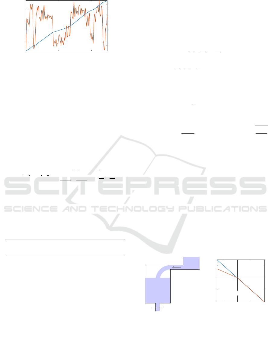
An abstract representation as a hydraulic model is
given in Figure 4. Two energy resources were consid-
ered: the aerobic energy resource (O) which is unlim-
ited in size but has a limited access rate called critical
power (P
C
) and the anaerobic energy resource (E
an
)
which is limited in size.
O
P
C
P
E
an
200 300 400 500
power (W)
-200
-100
0
100
P
C
Figure 4: Flow model of the Critical Power model (left) and
the rate of change in the anaerobic work capacity level for
a certain power output (right). The blue curve shows the
original critical power model while the red curve shows the
modified version with α = 0.5.
While the model originally was designed for con-
stant work rate exercise, a dynamic version is de-
rived easily from the hydraulic model. The change
Road Cycling Climbs Made Speedier by Personalized Pacing Strategies
111

˙e
an
of the remaining amount of fluid in the anaerobic
work capacity vessel is given by the difference of the
amount of fluid flowing into the vessel (P
C
) and the
amount of fluid leaving the vessel (P), P
C
− P.
First simulations indicated that the rate during re-
covery phases is too high in this classical model.
Therefore we modified it by damping the recovery
rate by a constant factor α. To get a smooth conjunc-
tion between recovery and exhaustion a tanh sigmoid
function as shown in Equation 4 was used.
˙e
an
= (P
C
− P)

1 − α
2
tanh

−
P
C
− P
20

+
1 + α
2

=: F
phys
(P)
(4)
Figure 4 shows the behavior of ˙e
an
for different power
outputs.
2.4.1 Parameter Estimation
The three parameters P
C
, E
an
and α of the physiologi-
cal model were determined with the step test and rides
I and II by assuming that the athlete was completely
recovered when the rides started and fully exhausted
at the end of each test.
Therefore parameters were chosen in a way that
the remaining anaerobic work capacity was zero at
the end of the rides by minimizing its squared error
as shown in Equation 5. To ensure that the remaining
anaerobic work capacity e
an
did not fall below zero
and did not exceed the anaerobic work capacity ves-
sels size E
an
during the rides the boundary conditions
in Equation 6 were added to the minimization prob-
lem.
min
3
∑
i=1
e
an,i
(T
i
)
2
(5)
0 ≤ e
an,i
(t) ≤ E
an
for i = 1,2,3 and t ∈ [0, T
i
]
(6)
e
an,1
(t), e
an,2
(t) and e
an,3
(t) are the remaining anaer-
obic work capacities during the step test, ride I and
ride II respectively and T
i
are the corresponding test
durations. The resulting parameters for each subject
are shown in Table 3.
2.5 Optimal Control Problem
In order to calculate an optimal strategy the time T
needed to complete a given course was minimized. To
avoid singular problems a regularization variable Q
was introduced. It is the derivative of the power P and
the regularization discourages large power variations.
This lead to the following optimal control problem.
Table 3: Physiological parameters of the subjects. The crit-
ical power P
C
, the anaerobic work capacity E
an
and the re-
covery damping factor α.
P
C
E
an
α
(W) (J)
subject 1 378 27465 0.10
subject 2 262 11999 0.49
subject 3 330 16432 0.63
subject 4 167 27038 0.16
subject 5 258 13789 0.20
subject 6 288 10616 0.11
Minimize the cost functional
J = T + ε
Z
T
0
Q(t)
2
dt
subject to the dynamic constraints
˙
P(t) = Q(t)
˙x(t) =
p
2e
kin
(t)/M
˙e
kin
(t) = F
mech
(e
kin
(t),x(t), P(t))
˙e
an
(t) = F
phys
(P(t))
the path constraints
0 ≤ e
an
(t) ≤ E
an
0 ≤ P(t) ≤ P
m
and the boundary conditions
x(0) = 0
x(T ) = x
f
e
kin
(0) = 0
e
an
(0) = E
an
where P(t), x(t), e
kin
(t) and e
an
(t) are the states, Q(t)
is the control, and x
f
is the length of the course.
This problem was solved numerically by the state-
of-the-art optimal control solver GPOPS-II (Patterson
and Rao, 2014).
3 RESULTS
Figure 5 shows the strategy chosen by subject 1 in
ride II as well as the calculated optimal strategy. Two
main differences in the strategies can be observed: In
the steep sections of the course the optimal strategy
suggests a higher power output than the athlete chose
whereas the athlete used this saved energy for a sprint
in the end.
In general we observe that the optimal strategy is
close to a constant power output with slightly higher
values for steep segments and lower values for flat
segments. Nearly all subjects chose a power output
lower than the optimal one in the first 10 km and fin-
ished the ride with a sprint. Only subject 5 selected
icSPORTS 2016 - 4th International Congress on Sport Sciences Research and Technology Support
112

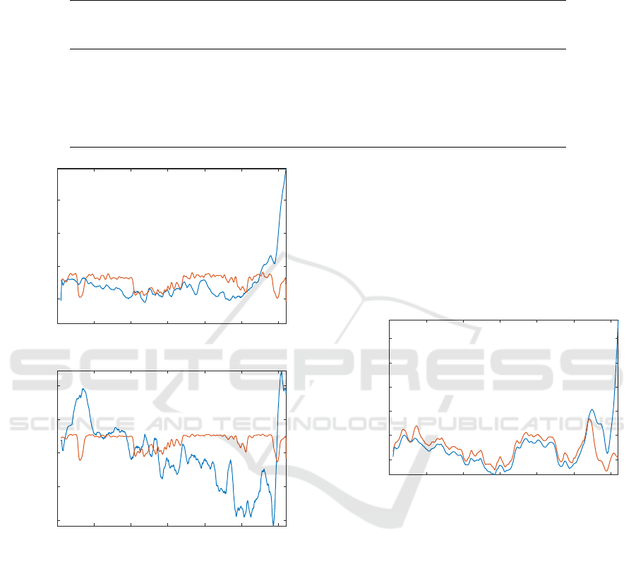
Table 4: Total race-times for the self-paced rides II, rides III with optimal strategy feedback and the validation rides IV. There
were no significant differences between the calculated optimal race-times and those of rides III. Additionally for rides III
the improvement compared to rides II is provided in relative values as well as whether the subjects were able to follow the
validation feedback in rides IV.
ride II ride III ride IV
self-paced optimal feedback validation feedback
(hh:mm:ss) (hh:mm:ss) (%) (hh:mm:ss) (target time achieved)
subject 1 00:43:03 00:42:43 -0.77 00:42:43 yes
subject 2 01:00:12 00:59:26 -1.27 00:59:26 yes
subject 3 00:44:28 00:43:55 -1.24 00:44:44 no
subject 4 01:19:01 01:16:51 -2.74 01:18:42 no
subject 5 00:58:17 00:57:00 -2.20 00:57:49 no
subject 6 00:53:55 00:52:10 -3.24 00:52:10 yes
0 2 4 6 8 10 12
distance (km)
380
400
420
440
power (W)
0 2 4 6 8 10 12
distance (km)
240
250
260
270
280
power (W)
Figure 5: Power output for subject 1 (top) and subject 5
(bottom). The red curve is the calculated optimal power
output and the blue curve is the power output during ride II
smoothed with a Gaussian filter (σ = 150 m).
a different strategy by starting with a high power out-
put, decreasing it during the ride and finishing with a
sprint (Figure 5).
In the ride with optimal strategy feedback, all sub-
jects were able to maintain the proposed strategy and
finish with the time the optimal strategy predicted.
This resulted in a reduction of the total race time com-
pared to the self-paced ride II (Table 4). The rela-
tive improvement was between 0.8 % and 3.2% cor-
responding to time savings between 20s and 130 s.
Three out of six subjects (1, 2 and 6) were able
to follow the validation strategy feedback and thus
exactly achieved the target finishing time identical to
that for the optimal pacing strategy. The other three
riders (3, 4 and 5) failed in that regard, becoming too
exhausted to maintain the proposed power output in
the end of the ride. In Figure 6 this behavior is shown
for subject 4. Until 10 km the subject was able to per-
form constantly above ride II but after that the perfor-
mance dropped considerable.
0 2 4 6 8 10 12
distance (km)
160
180
200
220
240
260
power (W)
Figure 6: Power output for subject 4. The red curve is the
power output during ride IV and the blue curve is the power
output during ride II. Both are smoothed with a Gaussian
filter (σ = 150 m).
4 DISCUSSION
In this study we addressed three questions:
1. Is it even possible to maintain the proposed opti-
mal strategy?
2. Does the race time improve using optimal strategy
feedback?
3. If so, does the race time improve because of the
strategy or because of the fact that there is a pace
maker?
The first two questions can be answered positively.
All subjects were able to follow the optimal strategy
Road Cycling Climbs Made Speedier by Personalized Pacing Strategies
113

until the end and the total race times improved for all
subjects compared to their own paced rides.
To answer the third question the subjects per-
formed ride IV. The feedback in ride IV implied a
power output constantly above the power output of
ride II. Since ride II was until exhaustion, it should
have not been possible to maintain the proposed
power output until the end of the ride.
Three out of six subjects confirmed this assump-
tion. They were not able to follow the feedback given
in ride IV in the last part of the race. Nevertheless the
other three subjects were able to maintain the strategy
until the end. This indicates that the feedback itself
motivated them to access more energy resources than
in their self paced ride.
Therefore question three cannot be answered
clearly. Feedback alone enabled most subjects to im-
prove their race times, even if they were not able to
follow it until the end. But the three subjects that
could not follow the feedback in ride IV until the end
clearly showed that there is a definite advantage using
the optimal strategy.
In order to answer the third question satisfacto-
rily and distinguish between improvements due to the
strategy and improvements due to the pace maker, a
larger set of participants would be needed to be able
to apply statistical methods and provide an adequate
quantitative justification.
5 CONCLUSIONS
Our experiment showed that the calculated optimal
strategy is feasible in a way that all athletes were able
to follow it until the end. Furthermore, it provides an
advantage over the strategy the athletes chose on their
own.
Even though external feedback itself already en-
abled most subjects to improve their performance, a
well chosen strategy like the calculated optimal strat-
egy is required to ensure that the athlete can finish the
race properly and enhance the total race time.
The next step to get closer to real racing conditions
is to perform a similar experiment in the field. There-
fore a feedback device has to be developed, which
incorporates a pace maker based on GPS measure-
ments.
Another major challenge arising with field tests is
to consider wind conditions along the track and to
provide a corresponding real-time adaptation of the
optimal strategy.
REFERENCES
Dahmen, T. and Brosda, F. (2016). Robust computation
of minimum-time pacing strategies on realistic road
cycling tracks. In Sportinformatik 2016, 11. Sym-
posium der dvs-Sektion Sportinformatik, Magdeburg,
Germany. accepted.
Dahmen, T., Byshko, R., Saupe, D., R
¨
oder, M., and
Mantler, S. (2011). Validation of a model and a simu-
lator for road cycling on real tracks. Sports Engineer-
ing, 14(2-4):95–110.
Dahmen, T., Wolf, S., and Saupe, D. (2012). Applications
of mathematical models of road cycling. IFAC Pro-
ceedings Volumes, 45(2):804–809.
Gordon, S. (2005). Optimising distribution of power during
a cycling time trial. Sports Engineering, 8(2):81–90.
Martin, J. C., Milliken, D. L., Cobb, J. E., McFadden, K. L.,
and Coggan, A. R. (1998). Validation of a mathemat-
ical model for road cycling power. Journal of applied
biomechanics, 14:276–291.
Monod, H. and Scherrer, J. (1965). The work capacity of a
synergic muscular group. Ergonomics, 8(3):329–338.
Morton, R. H. (1986). A three component model of hu-
man bioenergetics. Journal of mathematical biology,
24(4):451–466.
Morton, R. H. (1996). A 3-parameter critical power model.
Ergonomics, 39(4):611–619.
Patterson, M. A. and Rao, A. V. (2014). Gpops-ii: A mat-
lab software for solving multiple-phase optimal con-
trol problems using hp-adaptive gaussian quadrature
collocation methods and sparse nonlinear program-
ming. ACM Transactions on Mathematical Software
(TOMS), 41(1):1.
Sundstr
¨
om, D., Carlsson, P., and Tinnsten, M. (2014). Com-
paring bioenergetic models for the optimisation of
pacing strategy in road cycling. Sports Engineering,
17(4):207–215.
icSPORTS 2016 - 4th International Congress on Sport Sciences Research and Technology Support
114