Computing Ideal Number of Test Subjects

Sensorial Map Parametrization

Jessica Dacleu Ndengue

, Mihaela Juganaru-Mathieu

and Jenny Faucheu

Laboratoire Georges Friedel, Ecole Nationale Suprieure des Mines, F-42023 Saint Etienne, France

Department d’Informatique, Ecole Nationale Suprieure des Mines, F-42023 Saint Etienne, France

Keywords:

Napping

, Sensorial Map, RV-cofﬁcient.

Abstract:

A sensory analysis was carried using a special Napping

 table on two different set of products in order to

investigate on texture perception of material, the tests were done using a human panel. The data collected

were analyzed through multiple factor analysis (MFA) which is a particular case of principal component

analysis (PCA). The aim of this study is to know the minimum number of subjects in the human panel that

can guarantee a meaningful statistical analysis of data, and so far allows a better understanding of the sensory

results. We built a particular function that measures the similarity between two representations (two matrices)

which are computed using the output of Napping

 table. Based on this function and using the whole datasets

an algorithm able to measure the robustness is implemented. We found on the two datasets that a minimum

number of subjects between 10 and 12 seems to insure a stable and robust statistical analysis of the sensory

results.

1 INTRODUCTION

Projective mapping was introduced in 1994 (Risvik

et al., 1994) as a method in the ﬁeld of sensory sci-

ence, in the aim to collect similarities or dissimilari-

ties between products of the same type. The monog-

raphy (Varela and Ares, 2014) is a complete about

the subject. This procedure of projective mapping

is validated for food, beverage and fragrance prod-

uct (Kennedy and Heymann, 2009; Pag

es, 2003)

Napping

procedure, that is particular case of

projective mapping, was proposed by (Pag

es, 2003)

and R libraries FactoMiner (L

e et al., 2008) and

SensoMineR (L

e and Husson, 2008) were imple-

mented. The idea is to ask to some subject to place

in a space various sample of a generical product. The

number of samples is quite low, between 8 et 20 de-

pending of the type of the product and because it is an

human who manipulates these in a physical bounded

space. The number of subjects or assesors used in

all these experience is variable from 8 to more of

50. In (Kennedy and Heymann, 2009; Dehlholm

et al., 2012) clear synthesis of projective mapping

were done.

Based on (Faucheu et al., 2015) we are studying

the use of this procedure for the evaluation of materi-

als (Dacleu Ndengue et al., 2016), especially the tex-

ture of those materials required some investigation, in

order to validate the method for this type of product.

Because almost all the information about the percep-

tion of the product space relies on this, one of the es-

sential points refers to the number of subject that is

necessary to achieve a stable analysis. As said be-

fore, Napping has previously been used for food, bev-

erage and fragrance product; for those studies, differ-

ent number of subject were use, from 8 (Risvik et al.,

1997) to 83 (Barcenas et al., 2004). The main reason

of the difference in number of subject was that it de-

pend on the nature of the product space. Until now, no

research has concluded on a minimum number of sub-

jects that can provide a stable representation of prod-

uct space. For this reason, it appear very important

to investigate on that minimum number, in particular

because the use of napping for material evaluation is

not very common.

The work presented in this paper focused on two

main aspects. First of all, a strategy that investigates

on the inﬂuence of a subject on the global representa-

tion of the product space display on the mean repre-

sentation of sample. Secondly, a strategy that inves-

tigates on the minimum number of subject necessary

to achieve a stable mean representation of the product

space.

In the second section we will describe our data, the

Ndengue, J., Juganaru-Mathieu, M. and Faucheu, J.

Computing Ideal Number of Test Subjects - Sensorial Map Parametrization.

DOI: 10.5220/0006086404370442

In Proceedings of the 8th International Joint Conference on Knowledge Discovery, Knowledge Engineering and Knowledge Management (IC3K 2016) - Volume 1: KDIR, pages 437-442

ISBN: 978-989-758-203-5

437

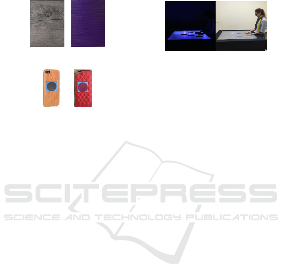
Figure 1: Image of one sample WC and one sample of

replica R.

Figure 2: Image of two sample of smartphone cover case

and their materials.

section 3 will explain the details about experiments,

collected dataset, statistical analysis, RV-coefﬁcient

which is important for our approach and the algo-

rithms we proposed. The results of evaluation are

given in section 4. In the last section some conclu-

sions are presented.

2 DATASETS

Two product spaces were use in this study. Those

samples were used in a sensory study aims at investi-

gating on texture perception of materials.

2.1 First Product Space: Wood

Countertype and Their Replica

We take into account 9 samples for the Wood Coun-

tertype (WC) and 9 samples for the replica (R), see

Figure 1. 18 untrained subjects participated to a sen-

sory analysis aimed at determining if familiarity af-

fects visual, tactile and visio-tactile perception of the

texture. This ﬁrst product space generated 6 datasets.

2.2 Second Product Space: Smartphone

Cover Case and Materials

12 Smartphone cover case for which texture was stud-

ied in order to determine how does the texture percep-

tion change according to the sample presentation. 23

untrained subjects took part to the experiment. The

samples were tested inform of material and in form of

object. So, two datasets are generated.

Finally, 8 datasets were obtained from these prod-

uct spaces and were analyzed in the study.

Tacti le (test Visual(and(Visuo-tac til e test

Figure 3: NappOmatic set-up for tactile, visual and visuo-

tactile perception of surface textures.

3 METHODS

3.1 Sensory Analysis and Data

Collection

We used a NappOmatic table (Faucheu et al., 2015).

We present brieﬂy this setup and we explain also the

procedure for the subjects /assessors.

NappOmatic Setup

The sensory experiments in this study aims at col-

lecting insights on the tactile, visual and visuo-tactile

perception of the two sets of samples. The procedure

used here was adapted from Napping

 (Pag

es, 2003)

which is a descriptive method deriving from the pro-

jective mapping (Risvik et al., 1994) originally devel-

oped for food and beverages.

In projective mapping, panelists are asked to posi-

tion on a large sheet of paper the products according

to the products’ similarities and dissimilarities. Pro-

jective mapping serves as a simple and quick tech-

nique to obtain product inter-distances. We devel-

oped a custom-made setup NappOmatic to perform

projective mapping with samples of materials and tex-

tures under visual, tactile and visual-tactile condi-

tions (D’Olivo et al., 2013; Faucheu et al., 2015) .

The NappOmatic experimental set-up is displayed

on Figure 3. The mapping area was deﬁned as a

square of 93cm × 93cm. In visual and visuo-tactile

tests, the room lights are on. For tactile tests, the

room is dark and the table is equipped with UV back

lights that enable to see the sample holder silhouette

and position, without seeing the texture and details of

the sample surface.

In this setup, the assessor can easily perform a

tactile exploration of the sample surface and position

the sample on the table (Figure 4). The number of

samples should be limited in order to avoid any sen-

sory tiredness. The tabletop is made of a translucent

material and a camera installed under the table takes

a picture of the mapping surface at the end of each

test. The back of the samples are tagged with QR

KDIR 2016 - 8th International Conference on Knowledge Discovery and Information Retrieval

438

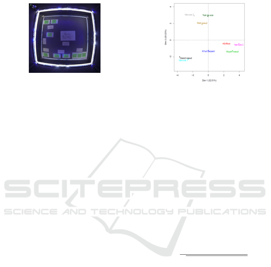
Figure 4: QR codes on the map.

code printed on ﬂuorescent paper to increase the con-

trast under UV light in order to enable the automatic

extraction of the sample positions using a software

speciﬁcally developed for this task.

For each assessor j, the data collected are the co-

ordinates (X

i j

) of each sample i and descriptors

associated to the samples by the assessors during the

experiment.

These data are processed through a Multiple Fac-

tor Analysis (MFA) implemented in the SensoMineR

software (L

e et al., 2008; L

e and Husson, 2008). MFA

is based on a Principal Component Analysis (PCA)

and have the advantage to allow the structuration of

the data in group to balance the inﬂuence of the as-

sessors in the analysis. From the MFA analysis, for a

given sensory modality, a mean representation of the

samples among the panel is extracted. In addition, the

descriptors cited by the assessors give indications on

how the samples were perceived and these descriptors

also give insights on the meaning of the axes deriving

from MFA.

Test Instructions

The assessors were instructed to arrange the samples

on the table, according to their perceived similarities

and differences. Samples that are perceived similar

should be close together, and those which are different

should be far from each other. After positioning the

samples, the assessors were asked to give attributes,

words that qualify their own perception of the texture

of each sample or group of samples. They were not

allowed to lift the sample from the table, but the ex-

ploration gestures were free.

3.2 Statistical Analysis with through

Mean Representation

For a given sample, for each assessor j, the data col-

lected have the coordinates (X

i j

, Y

i j

) of each sample

i and words associated to the samples by the subject.

Figure 5: A mean representation, it was obtained for WC

sample in visuo-tactile.

We ignore the words and we treated only the numeri-

cal data. These data are processed through MFA im-

plemented in the SensoMineR and FactomineR, (L

et al., 2008; L

e and Husson, 2008) packages of the

R software. From the MFA analysis, for a given sen-

sory modality, a mean representation of the samples

among the panel is extracted as in Figure 5.

A mean representation can be also represented as

a matrix of ﬁnal coordinate of the sample. Various

other techniques could be applied on this mean repre-

sentation like K-means or K-medoids or hierarchical

clustering.

3.3 RV-coeﬁcient

In (Robert and Escouﬁer, 1976) Robert and Escofﬁer

introduced the RV-Coefﬁcient in the aim to com-

pare two representations U and V in the same space.

In (Abdi, 2007) a deep analysis is done and we will

take the following formula :

RV =

trace(U

V )

trace(U

U)×trace(V

V )

RV-coefﬁcient is a measure of similarity of two

representations, like cosine in interval [0,1]. A value

near of 1 means very close representations, a small

value means different representations.

3.4 Algorithms

The common idea of both algorithms was to compute

the RV-coefﬁcient between the main representation of

the whole dataset (All) and the representation of a

part of dataset (Part). We note this function as RV ,

for example, RV (All, Part). We remember that All is

formed by the contributions U

of all the assessor j,

1 ≤ j ≤ N, where N is the number of assessors.

Computing Ideal Number of Test Subjects - Sensorial Map Parametrization

439

Contribution of an Assessor. The idea is to com-

pute RV (All, All \{U

}), for all j. So, the algorithm 1

which computes these values RV is quite simple:

Data: dataset All with the coordinates of the

samples indicated by each assessors

N ← size(All);

forall the j ∈ 1 : N do

coe f ← RV (All, All \ {U

})

end

Examine coe f

, j = 1, N

Algorithm 1: Algorithm to compute and the decide about

the importance of an assessor.

If we can see that all the assessor has an equivalent

importance, the natural question is how to ﬁnd a min-

imum number of assessors. In this aim, the following

algorithm 2 offers the possibility to decide which is

this minimum number. The algorithm generates for

every possible size k, k < N, a given number N

parts of All with cardinality k and for each part, we

compute its value of RV function, than we will take

into account only the min, the max and the average of

these values. The decision of the minimum number

of assessor will be taken examining the table of min,

max, average.

Data: dataset All with the coordinates of the

samples indicated by each assessors

N ← size(All);

← N − 1;

forall the k ∈ 2 : N − 1 do

forall the j ∈ 1 : N

P ← RandomPart(All, k);

← RV(All, All \ {U

})

end

min

← min(rv

);

max

← max(rv

);

avg

← average(rv

);

end

Examine min

, max

, avg

, j = 2, N − 1

Algorithm 2: Algorithm to compute and the decide about

the minimum number of assessors.

RandomPart(A,k) generates a random subset of A

having the cardinal k.

4 RESULTS

As said before, the RV coefﬁcient was calculated be-

tween different conﬁgurations, in order to analyze the

similarity and at the end, work out with the determi-

nation of the minimum number of subject that will

Table 1: The table of the assessors inﬂuence on the mean

representation for the smartphone cover case sample with

23 assessors.

Map without assessor RV coef p-value

1 0.9969245 9.647078e-06

2 0.9968665 7.686154e-06

3 0.9993329 7.652130e-06

4 0.9992873 7.316040e-06

5 0.9995793 7.969934e-06

6 0.9932582 1.222052e-05

7 0.9994813 8.492618e-06

8 0.9987969 8.993405e-06

9 0.9953651 6.763334e-06

10 0.9989282 6.687446e-06

11 0.9977334 8.360140e-06

12 0.9994534 7.552652e-06

13 0.9985761 7.457676e-06

14 0.9990266 6.415641e-06

15 0.9987920 7.058059e-06

16 0.9984504 7.141431e-06

17 0.9989072 6.864290e-06

18 0.9988803 8.242877e-06

19 0.9979545 6.610175e-06

20 0.9939960 1.494437e-05

21 0.9995917 8.265173e-06

22 0.9990081 8.223297e-06

23 0.9981801 9.765529e-06

guarantee a stable and statistically valid mean repre-

sentation that is related to the perception.

4.1 Individual Assessor

For the ﬁrst algorithm, for every dataset, the inﬂuence

of an assessor on the mean representation given by

RV-coefﬁcient was very close to 1, conﬁrmed by the

p-value, see table 1. This results conﬁrms that the in-

ﬂuence of each assessor is balanced in the mean rep-

resentation, and also every assessor has the same im-

portance in the experiments. This results conﬁrms the

reality : all the assessor had the same level of exper-

tise.

4.2 Minimum Assessors Number

For the R and WC datasets the results were analyzed

in every sensory modality: tactile, visual and visuo-

tactile. From various groups two to seventeen asses-

sors, the RV coefﬁcient was calculated between those

conﬁgurations and the one with the entire panel (18

subjects). As the procedure was performed 17 times

(for statistical validity), the mean value as well as

minimum, maximum were calculated. In addition, the

P-value of those RV coefﬁcient were also examine to

make sure the results are statistically signiﬁcant. Ta-

ble 2 display the results of the WC and R samples in

tactile, visual and visuo-tactile conditions.

KDIR 2016 - 8th International Conference on Knowledge Discovery and Information Retrieval

440

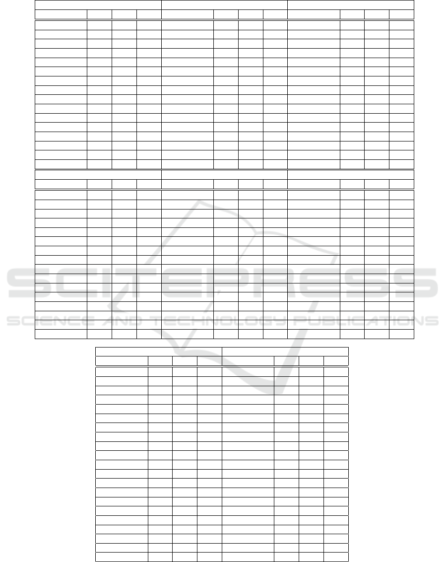
Table 2: The tables of RV values computed for WC datasets and for R datasets (up and middle) and for the datasets of

smartphones : cover case and material.

Tactile Visual Visuo-tactile

nb. assessors min moy max nb. assessors min moy max nb. assessors min moy max

2 0.46 0.62 0.76 2 0.57 0.76 0.9 2 0.55 0.67 0.8

3 0.62 0.73 0.81 3 0.59 0.8 0.86 3 0.62 0.75 0.83

4 0.62 0.79 0.89 4 0.7 0.85 0.92 4 0.7 0.78 0.84

5 0.77 0.83 0.91 5 0.74 0.88 0.94 5 0.68 0.82 0.89

6 0.72 0.85 0.92 6 0.86 0.91 0.95 6 0.75 0.84 0.91

7 0.84 0.89 0.94 7 0.87 0.93 0.96 7 0.82 0.89 0.93

8 0.83 0.9 0.94 8 0.85 0.94 0.98 8 0.83 0.91 0.95

9 0.88 0.92 0.96 9 0.89 0.94 0.98 9 0.86 0.91 0.96

10 0.87 0.93 0.97 10 0.93 0.96 0.97 10 0.89 0.93 0.96

11 0.92 0.95 0.97 11 0.94 0.96 0.98 11 0.91 0.94 0.96

12 0.92 0.96 0.98 12 0.94 0.97 0.98 12 0.92 0.95 0.98

13 0.94 0.96 0.99 13 0.95 0.97 0.99 13 0.91 0.96 0.98

14 0.95 0.97 0.98 14 0.97 0.98 0.99 14 0.95 0.97 0.98

15 0.95 0.98 0.98 15 0.98 0.98 0.99 15 0.93 0.98 0.99

16 0.98 0.99 0.99 16 0.98 0.99 0.99 16 0.97 0.98 0.99

17 0.98 0.99 0.99 17 0.99 0.99 0.99 17 0.98 0.99 0.99

Tactile Visual Visuo-tactile

nb. assessors min moy max nb. assessors min moy max nb. assessors min moy max

2 0.4 0.62 0.78 2 0.46 0.6 0.72 2 0.4 0.62 0.78

3 0.56 0.7 0.79 3 0.57 0.7 0.76 3 0.56 0.7 0.79

4 0.56 0.79 0.87 4 0.68 0.76 0.84 4 0.56 0.79 0.87

5 0.66 0.79 0.89 5 0.61 0.78 0.86 5 0.66 0.79 0.89

6 0.68 0.84 0.9 6 0.74 0.83 0.89 6 0.68 0.84 0.9

7 0.74 0.85 0.92 7 0.82 0.88 0.92 7 0.74 0.85 0.92

8 0.81 0.9 0.94 8 0.84 0.88 0.92 8 0.81 0.9 0.94

9 0.82 0.91 0.94 9 0.86 0.91 0.95 9 0.82 0.91 0.94

10 0.89 0.92 0.95 10 0.87 0.92 0.95 10 0.89 0.92 0.95

11 0.88 0.93 0.97 11 0.89 0.92 0.95 11 0.88 0.93 0.97

12 0.92 0.95 0.98 12 0.93 0.94 0.97 12 0.92 0.95 0.98

13 0.93 0.96 0.97 13 0.93 0.96 0.98 13 0.93 0.96 0.97

14 0.94 0.97 0.98 14 0.94 0.96 0.98 14 0.94 0.97 0.98

15 0.96 0.98 0.99 15 0.94 0.97 0.98 15 0.96 0.98 0.99

16 0.98 0.98 0.99 16 0.97 0.98 0.99 16 0.98 0.98 0.99

17 0.99 0.99 0.99 17 0.98 0.99 0.99 17 0.99 0.99 0.99

Smartphone cover case Sample material

nb. assessors min moy max nb. assessors min moy max

2 0.5 0.76 0.88 2 0.5 0.73 0.84

3 0.63 0.81 0.93 3 0.66 0.8 0.9

4 0.67 0.85 0.93 4 0.64 0.82 0.91

5 0.8 0.88 0.94 5 0.69 0.87 0.92

6 0.79 0.9 0.96 6 0.82 0.9 0.95

7 0.85 0.92 0.95 7 0.84 0.91 0.96

8 0.89 0.93 0.96 8 0.87 0.92 0.96

9 0.88 0.94 0.96 9 0.88 0.94 0.96

10 0.92 0.95 0.97 10 0.89 0.94 0.97

11 0.94 0.96 0.98 11 0.93 0.96 0.98

12 0.94 0.96 0.98 12 0.94 0.96 0.98

13 0.95 0.97 0.98 13 0.94 0.96 0.99

14 0.95 0.97 0.98 14 0.94 0.97 0.99

15 0.96 0.98 0.99 15 0.95 0.97 0.98

16 0.96 0.98 0.99 16 0.96 0.98 0.99

17 0.97 0.98 0.99 17 0.97 0.98 0.99

18 0.98 0.99 0.99 18 0.97 0.98 0.99

19 0.98 0.99 0.99 19 0.97 0.99 0.99

20 0.98 0.99 0.99 20 0.97 0.99 0.99

21 0.99 0.99 0.99 21 0.99 0.99 0.99

22 0.99 0.99 0.99 22 0.99 0.99 0.99

Computing Ideal Number of Test Subjects - Sensorial Map Parametrization

441

The minimum value of RV coefﬁcient was consid-

ered for better precision. On the view of those results,

it was observed that, for WC samples the similarity

with the global mean representation reaches 0.92 with

11 subjects; while for the R samples, it reaches 0.92

for 12 samples.

For the smartphone datasets, as for the WC and

R samples, the minimum RV coefﬁcient values were

analyzed. Those values expressing the similarity be-

tween the global mean representation of 23 assessors

and maps obtained with a number of assessors com-

prises between 2 and 22.

In the table 2 it can be observed that with 10 sub-

jects, the RV coefﬁcient reaches 0.92, so 10 is a min-

imum number of assessors.

5 CONCLUSIONS

In this paper we have used datasets collected for sen-

sorial analysis of materials. The questions solved are:

• how many subjects are necessary to realize a sig-

niﬁcant experience

• how could we prove that this minimal number is

correct

A methodology based on the use of a synthetic

value, in our case, the RV value, was described and

implemented. The method was applied on various

datasets and the obtained results proved the correct-

ness of our approach.

This methodology can be applied in other experi-

ences in the aim to optimize the sensorial map.

ACKNOWLEDGEMENTS

This work was supported by the LABEX

MANUTECH-SISE (ANR-10-LABX-0075) of

Universit

e de Lyon, within the program ”Investisse-

ments d’Avenir” (ANR-11-IDEX-0007) operated by

the French National Research Agency (ANR).

REFERENCES

Abdi, H. (2007). RV coefﬁcient and congruence coefﬁ-

cient. Encyclopedia of measurement and statistics,

pages 849–853.

Barcenas, P., Elortondo, F. P., and Albisu, M. (2004).

Projective mapping in sensory analysis of ewes milk

cheeses: A study on consumers and trained panel per-

formance. Food Research International, 37(7):723–

729.

Dacleu Ndengue, J., Faucheu, J., Bassereau, J.-F., Za-

houani, H., Massi, F., and Delafosse, D. (2016). Per-

ception of textured material: Does familiarity affects

tactile, visual and visuo-tactile discrimination? in

progress.

Dehlholm, C., Brockhoff, P. B., Meinert, L., Aaslyng,

M. D., and Bredie, W. L. (2012). Rapid descriptive

sensory methods–comparison of free multiple sort-

ing, partial napping, napping, ﬂash proﬁling and con-

ventional proﬁling. Food Quality and Preference,

26(2):267–277.

D’Olivo, P., Del Curto, B., Faucheu, J., Lafon, D.,

Bassereau, J.-F., L

e, S., and Delafosse, D. (2013).

Sensory metrology: when emotions and experiences

contribute to design. In 19th International Confer-

ence on Engineering Design (ICED13), pages DS75–

7 052. The Design Society.

Faucheu, J., Caroli, A., Del Curto, B., Delafosse, D., et al.

(2015). Experimental setup for visual and tactile eval-

uation of materials and products through napping



procedure. In DS 80-9 Proceedings of the 20th In-

ternational Conference on Engineering Design (ICED

15) Vol 9: User-Centred Design, Design of Socio-

Technical systems, Milan, Italy, 27-30.07. 15.

Kennedy, J. and Heymann, H. (2009). Projective mapping

and descriptive analysis of milk and dark chocolates.

Journal of Sensory Studies, 24(2):220–233.

e, S. and Husson, F. (2008). SensoMineR: A package

for sensory data analysis. Journal of Sensory Studies,

23(1):14–25.

e, S., Josse, J., Husson, F., et al. (2008). FactoMineR: an

R package for multivariate analysis. Journal of statis-

tical software, 25(1):1–18.

Pag

es, J. (2003). Direct collection of sensory distances: ap-

plication to the evaluation of ten white wines of the

loire valley. Sciences des Aliments, 23(5-6):679–688.

Risvik, E., McEwan, J. A., Colwill, J. S., Rogers, R., and

Lyon, D. H. (1994). Projective mapping: A tool for

sensory analysis and consumer research. Food quality

and preference, 5(4):263–269.

Risvik, E., McEwan, J. A., and Rødbotten, M. (1997). Eval-

uation of sensory proﬁling and projective mapping

data. Food quality and preference, 8(1):63–71.

Robert, P. and Escouﬁer, Y. (1976). A unifying tool for lin-

ear multivariate statistical methods: the rv-coefﬁcient.

Applied statistics, pages 257–265.

Varela, P. and Ares, G. (2014). Novel techniques in sensory

characterization and consumer proﬁling. CRC Press.

KDIR 2016 - 8th International Conference on Knowledge Discovery and Information Retrieval

442

REFERENCES

Abdi, H. (2007). RV coefficient and congruence coeffi-