Efficiency of the Equivalent Slab Thickness of the Ionosphere to Set

Radio Wave Propagation Conditions

Olga Maltseva and Natalia Mozhaeva

Institute for Physics, Southern Federal University, Stachki, 194, Rostov-on-Don, Russia

mal@ip.rsu.ru

Keywords: GPS, Total electron content TEC, Ionospheric models, Equivalent slab thickness.

Abstract: Now the total electron content ТЕС is a key parameter characterizing conditions of the ionosphere. ТЕС is

widely used for an estimation of positioning accuracy, definition of index of ionospheric storm activity. Data

of TEC is very important for systems of satellite communication and navigation. The advantages of the TEC

measurement are the systems of a large number of receivers, the possibility of continuous global monitoring

of the ionosphere, the availability of data on the Internet. For many systems (HF-communication, HFDF,

HFGINT) it is necessary to know the maximum density of the ionosphere NmF2 or, that is equivalent, a

critical frequency foF2. To obtain NmF2, it is necessary to know the proportionality coefficient

τ=TEC/NmF2, which is the equivalent slab thickness of the ionosphere. Before occurrence of navigational

satellites, no special attention was given to this parameter and there were many inaccuracies in the papers

devoted to τ. The possibility of the global monitoring of NmF2 with use of ТЕС, measured by navigational

satellites, makes to give the more close attention to its study. In the present paper, data of more than 50

ionospheric stations and several global maps of ТЕС are used to investigate behavior of a median τ(med) of

the observational equivalent slab thickness τ(obs). Comparison of τ(med) with the equivalent slab thickness

τ(IRI) of the IRI model, τ(NGM) of the Neustrelitz global model and others has shown essential differences

between these values. Approaches for developing a global model of τ(med) are offered. The most amazing

are following results: (1) for a large amount of stations, the use of observational TEC and τ(IRI) worsens

values of foF2 compared to the initial IRI model, (2) there are no fundamental quantitative differences in the

use of τ(med) for all regions of the world, (3) the IRI model and maps of TEC (in the absence of GPS receivers)

for the most northern Nord station (Greenland) showed surprisingly good agreement with the experimental

values of foF2.

1 INTRODUCTION

The critical frequency of the ionosphere foF2 was the

main parameter determining the state of the

ionosphere and radio wave propagation conditions in

the last century. It is connected with the maximum

density NmF2 of the ionosphere by the relationship

NmF2 = 1.24

10xfoF2

and with the maximum

usable frequency MUF through the propagation

factor M(D): MUF = M(D)xfoF2. This frequency is

measured by ground ionosondes. In the 21st century,

the total electron content TEC becomes the main

parameter. TEC is measured by means of navigation

satellites in units of TECU = 1

16 e/m

. The

advantages of the TEC measurement are regional

systems of a large number of receivers, the possibility

of continuous global monitoring of the ionosphere,

the availability of data on the Internet. Naturally,

there was a proposal to use TEC to determine the

maximum density of the ionosphere NmF2 and foF2.

To do this, we need to know the proportionality

coefficient τ=TEC/NmF2, which is the equivalent

slab thickness of the ionosphere. Despite the fact that

the measurement of NmF2 was begun with the

invention of ionosondes (Breit and Tuve, 1926) and

TEC measurements were begun with the first

artificial satellite launch (Aitchison and Weekes,

1959), and the opportunity to use τ to obtain

knowledge of the ionosphere parameters and the

atmosphere was immediately appreciated, interest in

this parameter was increased only with the advent of

satellite navigation systems GPS, GLONASS,

allowing measurement of TEC. Despite the huge

amount of publications, unified picture of the

behavior of the experimental equivalent slab

thickness τ(obs) does not exist because different data

Olga M. and Mozhaeva N.

Efﬁciency of the Equivalent Slab Thickness of the Ionosphere to Set Radio Wave Propagation Conditions.

DOI: 10.5220/0006226600050014

In Proceedings of the Fifth Inter national Conference on Telecommunications and Remote Sensing (ICTRS 2016), pages 5-14

ISBN: 978-989-758-200-4

is used to determine TEC. Distinctions concern both

technical characteristics, and heights of satellites.

Traditionally the International Reference Ionosphere

model IRI (Bilitza, 2001; Bilitza et al., 2014) and its

equivalent slab thickness τ(IRI) are used to calculate

foF2. However, on one hand, τ(IRI) is not an

empirical model in a statistical sense, but, on the other

hand, almost nobody compared values of τ(obs) and

τ(IRI) and suggested the use of experimental median

τ(med) to calculate foF2. In (Maltseva et al. 2011), it

was proposed to use τ(med) together with the

experimental values TEC(obs) and it was shown that

this use allows to obtain foF2 closer to the

experimental value foF2(obs) than by means of

τ(IRI), and to fill gaps of the experimental data of

foF2.

The aim of this article is to estimate: (1) the

features of the behavior of the median equivalent slab

thickness, (2) the effectiveness of its use together with

the total electron content to obtain the critical

frequencies in comparison with the equivalent slab

thickness of current models of the ionosphere, (3) the

opportunity of developing a global model of τ(med).

2 EXPERIMENTAL DATA AND

CALCULATED VALUES

The feature of the current stage of research is the

availability of online databases of experimental data

that allows us to obtain the results on a global scale

(Maltseva, 2015). Data of foF2 of 56 ionosondes of

vertical sounding were used together with 5 global

maps JPL, CODE, UPC, ESA, IGS (Hernandez-

Pajares et al., 2009). The disadvantage of ionospheric

data is their sketchy character however there are

stations for which long-term measurements are

available. Data of foF2 was taken from the databases

SPIDR (http://spidr.ngdc.noaa.gov/spidr/index.jsp) and

DIDBase (http://ulcar.uml.edu/DIDB/). TEC values

were calculated from IONEX files

(ftp://cddis.gsfc.nasa.gov/pub/gps/products/ionex/).

As models, we used IRI2001, IRI2012 (Bilitza, 2001;

Bilitza et al., 2014), which have the upper limit of

2,000 km, and IRI-Plas (Gulyaeva, 2003; Gulyaeva

and Bilitza, 2012) located on the site

http://ftp.izmiran.ru/pub/izmiran/SPIM/ and allowed

determining N(h)-profile up to heights of navigation

satellites h(GPS) by taking into account a

plasmaspheric part of the profile. The magnitude of

the equivalent slab thickness τ is calculated in

accordance with the relationship τ = TEC/NmF2 for

the model and experimental parameters TEC and

NmF2. In this paper, values of τ(IRI) of the IRI model

and the median τ(med) of observational τ(obs) are

calculated and compared. To evaluate the

effectiveness of their use jointly with observational

TEC(obs) we have introduced corresponding

efficiency coefficients. These coefficients are

determined by using the deviations of calculated foF2

from the observational foF2(obs). The value of

|ΔfoF2(IRI)=|foF2(obs) - foF2(IRI)| is the difference

between the instantaneous values of the IRI model

and observational foF2(obs). Monthly averages were

calculated. This difference is in the denominators of

the efficiency coefficients. |ΔfoF2(τ(IRI))|=

|foF2(obs)-foF2(τIRI)| is the difference between the

values calculated using τ(IRI) and TEC(obs) and the

observational foF2(obs). Deviation |ΔfoF2(τ(med))|=

|foF2(obs)-foF2(τmed)| is the difference between

values calculated using τ(med) and TEC(obs) and

foF2(obs). Coefficient KτIRI =| foF2(ΔIRI|) /

|ΔfoF2(τ(IRI))| is the coefficient of efficiency of joint

use of τ(IRI) and TEC(obs). Coefficient

of efficiency of joint use of τ(med) and TEC(obs).

These coefficients are given together with the line K

= 1 to visually evaluate the effectiveness of using

TEC(obs): if the coefficient is 1, this means that the

use of TEC(obs) leads to the same results of foF2, as

the initial IRI model without TEC(obs). In this case

|ΔfoF2(IRI)|=|ΔfoF2(τ(IRI))|. If the coefficient > 1,

then the use of TEC(obs) leads to results better than

the initial model. If the coefficient is higher than 1,

then the use of TEC(obs) worsens the results of the

model. These values determine how strongly the

deviation of the initial model differs from the

deviation of values calculated using τ(IRI) and

τ(med) together with TEC(obs).

3 FEATURES OF τ BEHAVIOR

In the literature, there are certain disagreements in the

describing of such features of τ as: 1) diurnal

variation, 2) seasonal variation, 3) latitudinal

dependence 4) dependence on solar activity, 5)

behavior during disturbed conditions. The most

important disagreement is the absence or weakness of

the latitudinal dependence of τ, noted in many

publications (Kouris et al., 2008; Sardar et al., 2012;

Vryonides et al., 2012). Real situation is given in

Figure 1.

If the latitudinal dependence of τ(med) was

absent, the value of τ(med) for one station could be

used in obtaining foF2 with the observational TEC in

Fifth International Conference on Telecommunications and Remote Sensing

the whole region. Of particular importance is the

study of the behavior of τ(obs) during disturbances

because it is different from the behavior of τ(med). In

paper (Maltseva et al. 2011), a hyperbolic

approximation of τ was introduced as τ(hyp) = b0 +

B1/Nm to build a regression relation in which Nm =

foF2 * foF2 (foF2 in MHz). Such function is

calculated for each map. An example is shown in

Figure 2. Approximation of τ(hyp) was built for a

more accurate determination of τ during the

disturbances.

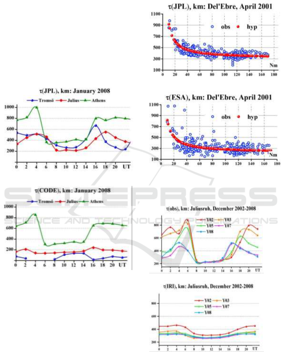
Figure 1. Example of the diurnal variation of τ(obs) for the

different latitude and two maps JPL and CODE.

The most important is the difference between

τ(IRI) and τ(med). Numerous examples are given in

papers (Maltseva and Mozhaeva, 2014, 2015) for

stations in all regions of the world with long-term

data. Example for the etalon station Juliusruh is

shown in Figure 3.

Large difference is seen not only in magnitude but

also in the diurnal variation. Namely this difference

determines the difference of the critical frequency

foF2(rec) reconstructed from the observational values

TEC(obs) using τ(med) and τ(IRI).

Figure 2: An example of a hyperbolic dependence of τ for

the disturbed month.

Figure 3: Differences of the model and the experimental

equivalent slab thicknesses in the example for the mid-

latitude station Juliusruh of European region and JPL map.

Efficiency of the Equivalent Slab Thickness of the Ionosphere to Set

Radio Wave Propagation Conditions

4 EFFICIENCY OF JOINT USING

τ(IRI) AND τ(MED) AND

TEC(OBS)

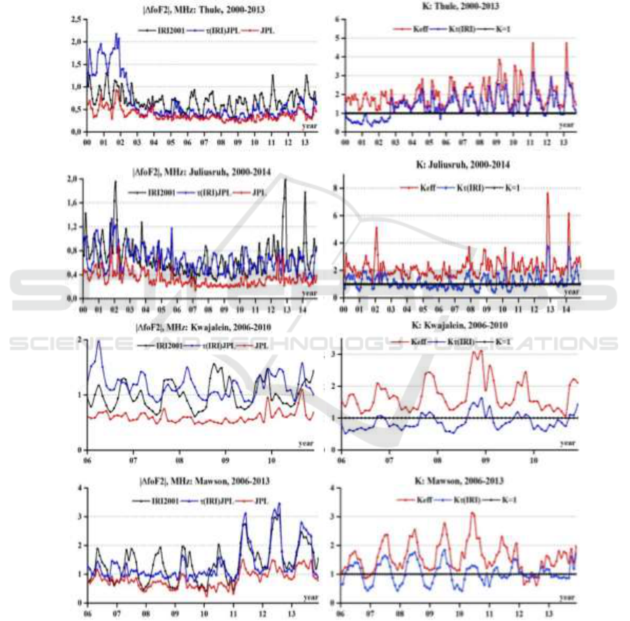
Figure 4 shows the deviation of the calculated values

of foF2 from foF2(obs) and efficiency coefficients for

stations with long-term observations: high- latitude

Thule, mid-latitude Juliusruh and equatorial

Kwajalein stations of the northern hemisphere and the

high-latitude Mawson station of the southern

hemisphere. Black dots show the results for the IRI

model, triangles present the results of joint using

τ(IRI) and TEC(obs), circles give the results of joint

using τ(med) and TEC(obs).

Figure 4: Deviations |ΔfoF2| and efficiency coefficients for the IRI model and two cases of using τ(IRI) and τ(med) together

with the TEC(obs).

It can be seen that the joint use of τ(IRI) and

TEC(obs) (K<1) can significantly worsen the

calculation of foF2 compared with the model (K <1).

By using τ(med) and TEC(obs) deviations |ΔfoF2| do

Fifth International Conference on Telecommunications and Remote Sensing

not exceed 1.0 MHz in most cases even in

problematic areas, such as high and equatorial

latitudes, and the coefficients are always exceed 1. In

the previous 2-3 years, a large amount of ionospheric

data has become available. This allows us to check

and compare the results simultaneously on many

stations on a global scale, in particular, to obtain these

results in the points in which they have not been

obtained and the IRI model was not tested itself. We

selected April 2014 and March 2015, because they

included geomagnetic disturbances.

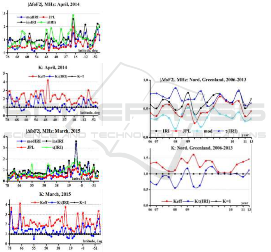
Figure 5: Correspondence between the model and the

observational values of foF2 and efficiency coefficients on

a global scale in April 2014 and March 2015.

Figure 5 illustrates the effectiveness of using

τ(med) globally by example of data for April 2014

(minimum Dst = -81 nT) and March 2015 (minimum

Dst = -223 nT). The samples shown on the x axis are

with a variable step, as stations are located not

uniformly.

It is evident that in the northern hemisphere the

amount of stations is larger than in the southern one.

In all cases, the use of τ(med) and TEC(obs) improves

matching calculated foF2(rec) with foF2(obs)

compared with two options: using the initial IRI

model and joint using τ(IRI) and TEC(obs). Joint

using τ(IRI) and TEC(obs) may provide poor results

compared to the initial model. The best results were

obtained for mid-latitudes. For high latitudes they

were not worse, but in the equatorial latitudes

problems for the model are seen, although the joint

use of τ(med) and TEC(obs) mitigates these

problems. Figure 6 gives the results for the Nord

station (Greenland) which are of particular interest

because it is the most northern station. Unfortunately

data of this station in the DIDbase were downloaded

recently and in a very limited extent (a few months

and not each year).

Figure 6: Long-term statistics for the Nord station

(Greenland) for available months of years indicated on the

x axis.

The results are almost similar to the results for

Thule, Tromso and other lower high-latitudinal

stations. Since the critical frequency of the Nord

station has never been compared with the model the

upper-hand plot of Figure 6 presents the curve

showing the deviation of the model from the

experimental medians of foF2. Results indicate a

surprisingly good performance of the IRI model in

this region.

Efficiency of the Equivalent Slab Thickness of the Ionosphere to Set

Radio Wave Propagation Conditions

5 ABOUT THE CONSTRUCTION

OF A GLOBAL MODEL OF

τ(MED)

The mention of the opportunity to construct a model

of τ is practically absent in the papers, but in recent

years some articles were published on the use of TEC

and the ionospheric equivalent slab thickness τ to

determine NmF2, what confirms the importance of

this problem. In (Gerzen et al., 2013), the authors

have proposed the use of two Neustrelitz models of

TEC and NmF2 (Hoque and Jakowski, 2011;

Jakowski et al., 2011) for the calculation of foF2, but

without sufficient testing. We use these models under

one name NGM (from Neustrelitz Global Model). It

is obvious that authors of (Gerzen et al., 2013) have

also used the value of τ(NGM) = TEC(NGM)/NmF2,

which can serve as an empirical model of τ. However,

testing this model in (Maltseva et al., 2013, 2014)

showed that in many regions the value of τ(NGM) is

very different from the experimental τ(med). In

(Muslim et al., 2015), a model of the average values

of τ was proposed as expansion in Fourier series

according to the TEC of the global map CODE and

foF2 for 21 stations, however, the assumptions made

in constructing the model: (1) linear dependence of all

parameters of the TEC, foF2 and τ on solar activity,

(2) lack of longitudinal dependence of these

parameters at the same local time LT, (3) regularity

of τ in quiet and disturbed conditions need

confirmation. This allows drawing a conclusion about

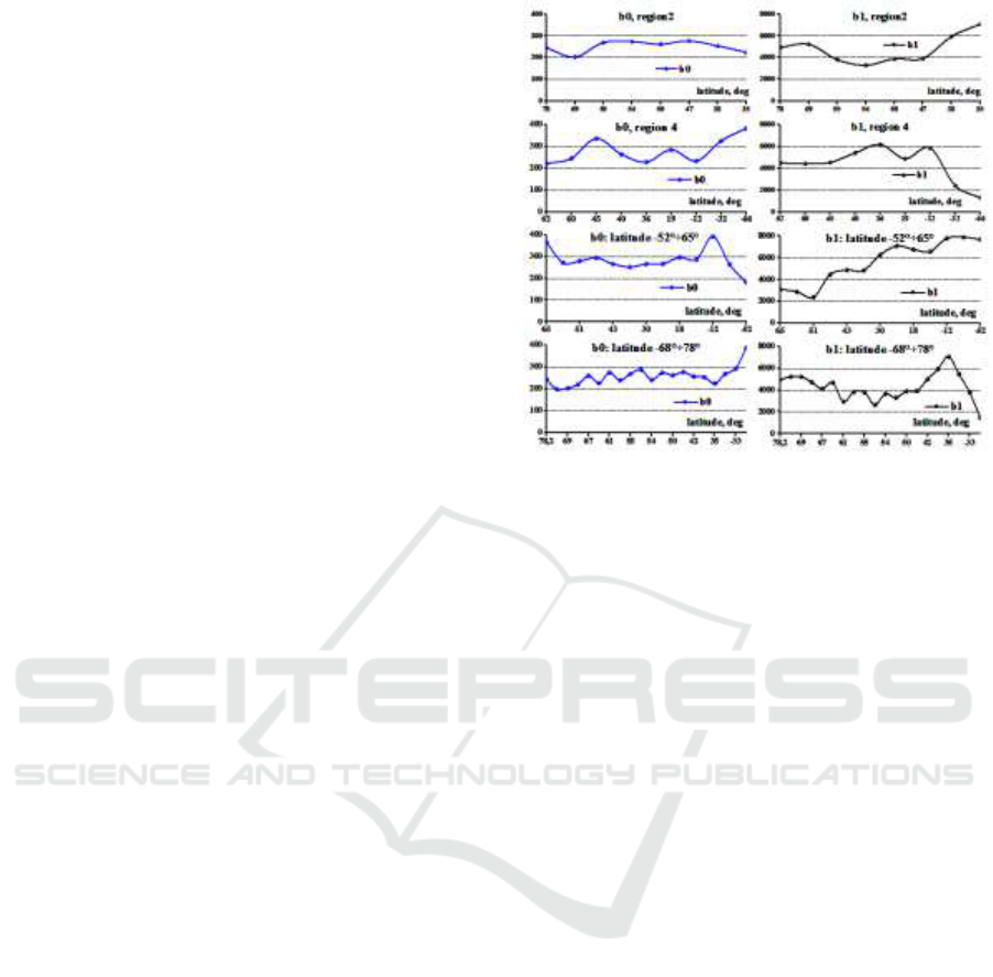
the need to develop the model of τ. To build a model

of τ(med) on a global scale two approaches are

proposed: two-parameter model based on a

hyperbolic approximation τ(hyp) = b0 + b1/NmF2

and the use of the coefficient K(τ)= τ(med)/τ(IRI),

since the construction of the model using the values

themselves is not possible because of the large

variability of values (in particular, the pre-sunrise

peak on some latitudes). A hyperbolic dependence

and approximation coefficient K(τ) were calculated

for March 2015. The results are shown for two

regions 2 (15°E <λ <40°E) with 8 stations and 4

(110°E <λ <170°E) with 9 stations and two wider

zones (Lat1 and Lat2). Area Lat1 includes stations,

located mostly in American continent of northern and

southern hemispheres. Area Lat2 includes stations

from European, Siberian and South-Eastern regions.

Behavior of coefficients b0 and b1 is shown in Figure

7 for these regions.

The test results of this model are shown in

Table_1

Figure 7: Behavior of hyperbolic approximation

coefficients in various regions

Table 1 includes different deviations. Column 1

indicates the station name and the region to which it

belongs. The second column shows the coefficients

of the hyperbolic approximation of τ(obs) for the

corresponding station. The third column specifies

conditions to which the two rows of values belong.

The top line (full) indicates average for all days of the

month, the bottom line (dist) gives average for

disturbed days (from 16 to 21 March). The fourth

column shows the results for the initial IRI model, the

fifth column presents the absolute difference between

the foF2(obs) and the values calculated using τ(med)

and TEC(obs). Column 6 contains the frequency

deviation, calculated using the coefficients b0 and b1

of the hyperbolic approximation for a given station.

The remaining columns give results of using

coefficients of areas referred to in the line title. All of

these values should be compared with the values for

the IRI model in bold. This is a test of the

effectiveness of the model. It can be seen that all

values are higher in disturbed days and the largest

differences concern to the initial IRI model. It is seen

that frequencies of one region could be used to

calculate the coefficients for other region. This

demonstrates a global character of the model of

τ(med).

Another method of constructing a global model of

τ(med) would be to use the coefficients K(τ)=

τ(med)/τ(IRI). Definite advantage of this model

might be in the fact that its denominator is the value

of τ(IRI), which has a global character, and a small

change in K(τ) in areas with close latitudes.

The distinction is development of a model for

each hour. The degree of proximity of τ is better

Fifth International Conference on Telecommunications and Remote Sensing

illustrated in the circular diagram. An example of

some diagrams is shown in Figure 8 for region 4 for

UT = 0, 6, 12, and 18 on March 2015. The red line

shows the value of coefficient K(τ), green triangles

are the average values, the blue quadrates concern

circles with radius R = 1.

Table 1: Deviation of frequencies, calculated by the hyperbolic dependence, from the experimental values in March 2015.

station

b1, b0

IRI

rec

stat

reg2

reg4

Lat1

Lat2

Juliusruh

3295.5

full

0.73

0.41

0.43

0.68

0.67

1.03

0.57

reg2

273.2

dist

1.44

0.52

0.49

0.67

0.68

1.07

0.64

Athens

5929.3

full

0.91

0.36

0.46

0.56

0.48

0.52

0.58

reg2

253.2

dist

1.31

0.44

0.74

0.52

0.59

0.87

0.51

Grahamstown

3788.7

full

0.80

0.40

0.54

0.77

0.59

0.73

Lat2

293.2

dist

1.54

0.46

0.62

0.84

0.75

0.82

0.77

Longyearbyen

4947.1

full

0.70

0.43

0.62

0.60

0.58

0.82

0.58

Lat2

244.2

dist

0.69

0.49

0.73

0.69

1.01

0.63

Thule

692.7

full

0.51

0.14

0.15

0.56

0.42

0.47

0.59

437.6

dist

0.55

0.10

0.13

0.51

0.46

0.64

0.54

Millstonehill

4864.4

full

0.90

0.50

0.47

0.48

0.46

0.67

0.49

Lat1

265.4

dist

1.38

0.67

0.65

0.81

0.80

Bejing

5402.8

full

1.17

0.49

0.61

0.58

0.70

0.62

reg4

263.9

dist

1.99

0.42

0.64

0.45

0.51

0.84

0.45

Kokubunji

6176.7

full

1.29

0.47

0.65

0.61

0.69

0.85

0.62

reg4

228.4

dist

2.11

0.55

0.66

0.56

0.70

0.96

0.56

Niue Island

4874.7

full

1.85

1.15

1.36

1.35

1.28

1.43

1.29

reg4

285.0

dist

1.67

0.71

1.00

0.73

0.85

1.11

0.67

Cocos Island

5467.3

full

1.43

0.55

0.68

0.86

0.62

0.65

0.82

Lat2

267.8

dist

1.66

0.52

0.77

0.88

0.67

0.80

0.83

Mawson

1466.2

full

0.91

0.27

0.37

1.00

0.85

1.02

0.92

Lat2

386.8

dist

1.12

0.12

0.21

0.80

0.98

0.81

Efficiency of the Equivalent Slab Thickness of the Ionosphere to Set

Radio Wave Propagation Conditions

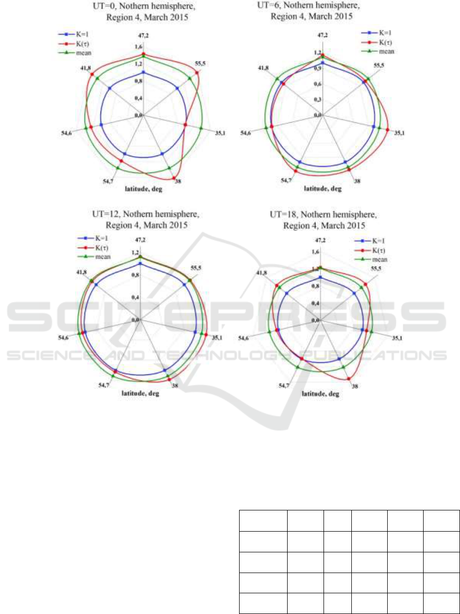
Figure 8: Illustration of charts for the coefficient K(τ).

The model is the average value K(mean). The

algorithm of its use is calculation of the new value

τ(Kτ) = K(mean) x τ(IRI) and the use of this new

value together with TEC(obs) to calculate foF2. To

test the efficiency of the algorithm, averages of

K(mean) were calculated for 7 stations for region

consisted of 8 stations and were used to calculate foF2

for the 8

station. Results are presented in Figure 9 as

deviations of the calculated values from observational

foF2(obs) for the four stations: Pruhonice,

Gorkovskaya, Tunguska and Ramey.

Table 2. Average deviations of calculated foF2 from

foF2(obs) using various options of models and τ.

station

IRI-

off

IRI-

τ(IRI)

new

τ(med)

Pruhonice

0.63

0.65

0.54

0.34

0.32

Gorkovsk

0.64

0.60

0.43

0.37

0.36

Tunguska

0.95

0.86

0.72

0.57

0.50

Ramey

0.78

0.85

1.36

0.78

0.58

Fifth International Conference on Telecommunications and Remote Sensing

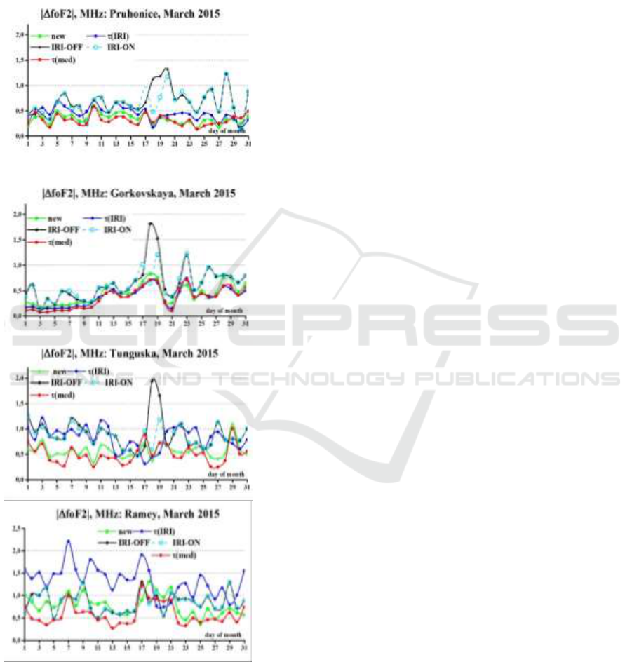
All plots contain curves of deviations for the

initial model without the use of TEC. Since both

options (off and on) were used, the curves were

indicated by IRI-off and IRI-on. Curves with the icon

τ(IRI) show results of joint using of τ(IRI) and

TEC(obs).

Figure 9: Deviation of calculated foF2 values from

foF2(obs) using various options of τ.

The curves marked by “new” show test values for

the Kτ model. Asterisks present results for τ(med) and

TEC(obs). Most values of |ΔfoF2| do not exceed 1

MHz. Significant deviations are only visible to the

IRI model in disturbed days on March 18-21 for the

case τ(IRI) and for the Ramey station. Quantitative

characteristics are given in Table. 2.

6 CONCLUSIONS

Data of more than 50 ionospheric stations and several

global maps of ТЕС were used to study behavior of a

median τ(med) of the observational equivalent slab

thickness τ(obs) and comparisons with existing

models τ(IRI), τ(NGM) and others. Essential

differences between them, leading to the large

deviations of the calculated values of foF2 from the

experimental ones are shown. As a quantitative

estimation, the effectiveness coefficients of joint

using TEC(obs) and τ(med) in comparison with joint

using TEC(obs) and τ(IRI) are used. It is shown that

the effectiveness coefficients practically always

exceed 1 for joint using of TEC(obs) and τ(med).

There are several striking results: (1) for a large

amount of stations, the use of observational TEC and

τ(IRI) worsens values of foF2 compared to the initial

IRI model, (2) there are no fundamental quantitative

differences in the use of τ(med) for all regions of the

world, (3) the IRI model and maps of TEC (in the

absence of GPS receivers) for the most northern Nord

station (Greenland) showed surprisingly good

agreement with the experimental values of foF2. In

this sense, results of HF propagation modeling on

high-latitude paths based on the IRI model

(Blagoveshchensky et al., 2016) seem no longer

surprising. Two approaches for developing a global

model of τ(med) are offered.

ACKNOWLEDGEMENTS

The authors thank the scientists who provided data of

SPIDR and DIDBase, global maps of TEC, operation

and modification of the IRI model, Southern Federal

University for financial support (grant N 213.01-

11/2014-22).

REFERENCES

Aitchison, G.J., Weekes, K., 1959. Some deductions of

ionospheric information from the observations of

emissions from satellite 1957α2—I: The theory of the

analysis, J. Atm. Terr. Phys., 14(3–4), 236–243.

doi:10.1016/0021-9169(59)90035-2.

Efficiency of the Equivalent Slab Thickness of the Ionosphere to Set

Radio Wave Propagation Conditions

Bilitza, D., 2001. International Reference Ionosphere,

Radio Sci., 36(2), 261-275.

Bilitza, D., Altadill, D., Zhang, Y., Mertens, C., Truhlik, V.,

Richards, P., McKinnell, L.-A., Reinisch, B., 2014.The

International Reference Ionosphere 2012 – a model of

international collaboration, J. Space Weather Space

Clim., 4, A07, 12p. DOI: 10.1051/swsc/2014004.

Blagoveshchensky, D.V., Maltseva, O.A., Anishin, M.M.,

Rogov, D.D., Sergeeva, M.A., 2016. Modeling of HF

propagation at high latitudes on the basis of IRI, Adv.

Space Res., 57, 821–834.

Breit, G., Tuve, M.A., 1926. A test for the existence of the

conducting layer, Phys. Rev., 28, 554-575.

Gerzen, T., Jakowski, N., Wilken, V., Hoque, M.M., 2013.

Reconstruction of F2 layer peak electron density based

on operational vertical total electron content maps, Ann.

Geophys., 31, 1241-1249. doi:10.5194/angeo-31-1241-

2013.

Gulyaeva, T.L., 2003. International standard model of the

Earth’s ionosphere and plasmasphere, Astron. and

Astrophys. Transaction, 22, 639-643.

Gulyaeva, T., Bilitza, D., 2012. Towards ISO Standard

Earth Ionosphere and Plasmasphere Model, In: New

Developments in the Standard Model, (R.J. Larsen ed.).

NOVA, Hauppauge, New York, 1–48.

Hernandez-Pajares, M., Juan, J. M., Orus, R., Garcia-Rigo,

A., Feltens J., Komjathy, A., Schaer, S.C., Krankowski,

A. 2009. The IGS VTEC maps: a reliable source of

ionospheric information since 1998, J. Geod., 83, 263–

275.

Hoque, M.M., Jakowski, N., 2011. A new global empirical

NmF2 model for operational use in radio systems.

Radio Sci., 46, RS6015, 1-13.

Jakowski, N., Hoque M.M., Mayer C., 2011. A new global

TEC model for estimating transionospheric radio wave

propagation errors, J. Geod., 85(12), 965-974.

Kouris, S.S., Polimeris, K.V., Cander, L.R., Ciraolo L.,

2008. Solar and latitude dependence of TEC and SLAB

thickness, J. Atmos. Solar-Terr. Phys., 70, 1351-1365.

Maltseva, O.A., 2015. Usage of the Internet resources for

research of the ionosphere and the determination of

radio-wave propagation conditions. Proceedings of the

Fourth International Conference on

Telecommunications and Remote Sensing, Rhodes,

Greece, 17-18 September, 7-17.

Maltseva, O.A., Mozhaeva, N.S., 2014. Features of

behavior and usage of a total electron content in the

Indian region, International Journal of Engineering

and Innovative Technology,4(4), October 2014, 1-9.

www.ijeit.com, ISSN: 2277-3754.

Maltseva, O.A., Mozhaeva, N.S., 2015. Obtaining

Ionospheric Conditions according to Data of

Navigation Satellites, International Journal of

Antennas and Propagation. 1-16.

http://dx.doi.org/10.1155/2015/804791.

Maltseva, O.A., Mozhaeva, N.S., Glebova, G.M., 2011.

Global maps of TEC and conditions of radio wave

propagation in the Mediterranean area, PIERS

Proceedings, Marrakesh, MOROCCO, March 20-23,

1Р9_0422, 1-5.

Maltseva, O.A., Mozhaeva, N.S., Nikitenko, T.V., 2014.

Validation of the Neustrelitz Global Model according

to the low latitude Adv. Space Res., 54 () 463–472.

Maltseva, O.A., Mozhaeva, N.S., Nikitenko T.V., 2015.

Comparative analysis of two new empirical models IRI-

Plas and NGM (the Neustrelitz Global Model), Adv.

Space Res., 55, 2086–2098.

Maltseva, O., Mozhaeva, N., Vinnik, E., 2013. Validation

of two new empirical ionospheric models IRI-Plas and

NGM describing conditions of radio wave propagation

in space. Proceedings of Second International

Conference on Telecommunications and Remote

Sensing, Noordwijkerhout, The Netherlands, 11-12

July, 109-118.

Muslim, B., Haralambous, H., Oikonomou, Ch.,

Anggarani, S., 2015. Evaluation of a global model of

ionospheric slab thickness for foF2 estimation during

geomagnetic storm. Ann. Geophys., 58(5), A0551.

doi:10.4401/ag-6721.

Sardar, N., Singh, A.K., Nagar, A., Mishra, S.D., Vijay,

S.K., 2012. Study of Latitudinal variation of

Ionospheric parameters - A Detailed report, J. Ind.

Geophys. Union, 16(3), 113-133.

Fifth International Conference on Telecommunications and Remote Sensing