Narrow Band Pressure Computation for Eulerian Fluid Simulation

Aditya Prakash and Parag Chaudhuri

Department of Computer Science and Engineering, Indian Institute of Technology Bombay, Mumbai, India

Keywords:

Eulerian Fluid Simulation, Narrow Band Pressure Solve, Fluid Animation.

Abstract:

An Eulerian ﬂuid simulation for incompressible ﬂuids spends a lot of time in enforcing incompressibility

by solving a large Poisson’s equation. This involves solving a large system of equations using a solver like

conjugate gradients. We introduce a way of accelerating this computation by dividing the grid domain of

the ﬂuid simulation into a narrow band of high resolution grid cells near ﬂuid-solid boundaries and a coarser

grid everywhere else. Judiciously reducing the number of high resolution grid cells signiﬁcantly lowers the

cost of the pressure projection step, while not sacriﬁcing the simulation quality. The coarse grid values are

upgraded to a ﬁner grid before advecting the ﬂuid surface so that enough degrees of freedom are available

to resolve surface detail. We present and analyse two methods to perform this upgradation, namely, velocity

interpolation and pressure ﬁeld smoothing. We discuss the merits and demerits of each and quantify the errors

introduced in the simulation as a function of size of the narrow band. Finally, since we are primarily interested

in visualizing the ﬂuid animation, we produce rendered ﬂuid simulation output to also validate the visual

quality of the simulations.

1 INTRODUCTION

Eulerian ﬂuid simulation involves solving the Navier-

Stokes equations on a ﬁxed grid. An incompressible

ﬂuid solve on a regular rectilinear grid is a common

example of this kind of simulation. Even in its sim-

plest setting this a computationally intensive task, and

a major proportion of this computation is spent in the

pressure projection stage that enforces ﬂuid incom-

pressibility (Lentine et al., 2010; Prakash and Chaud-

huri, 2015). This is done by solving a Poisson’s equa-

tion using an iterative or direct solver.

A lot of earlier research has attempted to in-

crease the speed of pressure projection on ﬁxed grids.

These methods are either not tailored for visual liq-

uid simulation (Montijn et al., 2006), or use speciﬁc

complicated grid structures (Ferstl et al., 2014), or

treat the ﬂuid free surface differently from rest of

the ﬂuid volume (Autodesk, ). Dimension reduction

techniques (Treuille et al., 2006) and different ba-

sis functions (De Witt et al., 2012) have also been

used for this purpose. The problem however, remains

challenging for liquids simulation as the ﬂuid vol-

ume topology changes rapidly and enforcing correct

boundary conditions is difﬁcult.

We speciﬁcally focus on visual ﬂuid (liquid) ani-

mation and present a technique to accelerate the pres-

sure solve by creating a very coarse grid for the en-

tire ﬂuid simulation, except for a narrow band of ﬁne

grid cells around the boundary. This grid structure

is statically determined and does not require runtime

re-gridding. It perfectly enforces both Dirichlet and

Neumann boundary conditions at the ﬂuid free sur-

face and ﬂuid-solid boundary. We avoid the pitfalls of

the previous methods while still managing to main-

tain enough degrees of freedom in the ﬁnal velocity

ﬁeld of the ﬂuid simulation so as to be able to gener-

ate adequate surface detail. Our speciﬁc contributions

are as follows:

1. We present a simple, ﬂexible method to reduce the

size of the pressure projection problem by using a

coarser grid and a narrow band ﬁne grid. We show

how to couple these together to enforce both free

surface and ﬂuid-solid boundary conditions.

2. We show how to upgrade values from the coarse

grid back to a ﬁne grid to get adequate degrees of

freedom in the velocity ﬁeld to represent surface

detail using two techniques, namely, velocity in-

terpolation and pressure ﬁeld smoothing.

3. We rigorously compare the speedups obtained

in computation while using the two upgradation

strategies. We also quantify the errors introduced

due to our methods, and the visual quality of the

simulation thus produced, in both 2D and 3D.

Prakash A. and Chaudhuri P.

Narrow Band Pressure Computation for Eulerian Fluid Simulation.

DOI: 10.5220/0006090200170026

In Proceedings of the 12th International Joint Conference on Computer Vision, Imaging and Computer Graphics Theory and Applications (VISIGRAPP 2017), pages 17-26

ISBN: 978-989-758-224-0

These ideas substantially reduce the computa-

tional cost of the pressure solve without compromis-

ing on simulation quality. Our method is also easy to

parallelize and works perfectly on multi-core archi-

tectures.

We start by looking at existing literature in the

concerned area in Section 2. We brieﬂy discuss the

details of the Navier-Stokes equation and the Pois-

son’s equation that requires most of the computational

effort to solve during the simulation in Section 3.

We follow this up with a detailed description of our

narrow band pressure solve method and all the algo-

rithms in Section 4. We compare the performance of

our algorithms, the visual and timings results obtained

and the errors involved in Section 5. We conclude in

Section 6 with a brief summary and discussion about

limitations of the current system and possible future

directions.

2 BACKGROUND

Grid-based Eulerian simulation of incompressible ﬂu-

ids is commonly used for visual ﬂuid animation in

computer graphics and scientiﬁc visualization. Many

authors have presented systems that present visually

compelling results from ﬂuid simulations on Eulerian

grids (Stam, 1999; Foster and Fedkiw, 2001; Enright

et al., 2002), however, the size of the grids that these

techniques can use is limited by computational power

available.

As a consequence of this, many authors have

looked at adding details to these simulations by

adding various kinds of noise, like Kolmogorov

noise (Larmorlette and Foster, 2002; Rasmussen

et al., 2003) or curl noise (Bridson et al., 2007). Some

techniques (Schechter and Bridson, 2008) determine

where to add the noise and couple it to the Navier-

Stokes equations. However, these are not physically

realistic techniques and do not produce convincing

details in all situations.

Another approach is to improve the original sim-

ulation by the particular choice of the methods used

to solve each stage depending on accuracy, stability

and computational cost. E.g. semi-Lagrangian ad-

vection, proposed by Stam et al. (Stam, 1999) is un-

conditionally stable but has only ﬁrst order accuracy,

whereas Selle et al. (Selle et al., 2008) used a modiﬁed

McCormack scheme to give second order accuracy to

the advection step. Another way is to try and main-

tain certain invariants like energy (Mullen et al., 2009)

during the simulation. These methods increase accu-

racy and ﬁdelity of the simulation, but they involve

more expensive computation and are still limited by

the grid resolution on which the simulation is per-

formed. In order to increase grid resolution without

too much computational cost, some authors have in-

troduced adaptive grid techniques like AMR (Berger

and Oliger, 1984) and octrees (Losasso et al., 2004),

however, these complicated data structures are difﬁ-

cult to update during simulation and robust numerical

solutions are difﬁcult to design on such grids.

Lentine et al. (Lentine et al., 2010) present a

method of using a multi-resolution grid to speedup

the pressure projection step. They also require the ve-

locity ﬁeld to be interpolated from a lower resolution

to a higher one. We show in this paper that velocity

interpolation is a poorer speedup strategy as forcing

the velocity ﬁeld to be divergence free is harder post

interpolation and leads to lower speedups than other

methods.

Other authors have presented multigrid techniques

for efﬁciently solving Poisson problems (McAdams

et al., 2010; Chentanez and M

uller, 2011; Jung et al.,

2013). Though theoretically multigrid techniques are

very efﬁcient, they require precise discretization and

complicated data-structures for correctly converging

on regular grids (Ferstl et al., 2014). Our method is

much easier to apply and is guaranteed to converge.

Ando et. al (Ando et al., 2015) describe the work

that is closest to ours in spirit. They also describe a

dimension reduction strategy for simplifying the pres-

sure solve. Their work uses an up-sampling matrix

to interpolate the pressure to a higher resolution grid

during the pressure solve. They enforce Dirichlet

boundary conditions by using a surface aware pres-

sure basis to make the pressure zero at the free sur-

face. Our method is closely related to this work in

that we too present a dimension reduction strategy in

that interpolates pressure to a higher resolution grid,

after the linear pressure solve. In addition we com-

pute pressure at higher resolution in a narrow band

around the ﬂuid-solid boundary. This gives a better

solution in this boundary region. Our method is also

easier to understand and implement.

Authors have also investigated hybrid Eulerian-

Lagrangian methods to achieve speedup in ﬂuid sim-

ulation computations. Chentanez et. al (Chentanez

et al., 2014) couple a Eulerian solver, a shallow water

solver and a Lagrangian SPH solver within a simula-

tion. The material point method (MPM) combines a

grid-based Eulerian simulation with marker particles

to simulate a range of materials like snow (Stomakhin

et al., 2013) and foams (Yue et al., 2015). Ferstl et.

al (Ferstl et al., 2016) present a solution for accelerat-

ing FLIP advection in Eulerian grid-based ﬂuid simu-

lations by using FLIP particles only in a narrow band

around the free surface of the ﬂuid.

GRAPP 2017 - International Conference on Computer Graphics Theory and Applications

Some authors have also experimented with addi-

tion of high resolution detail to low-resolution simu-

lations (Threy et al., 2010; Kim et al., 2013) but these

are largely orthogonal to the techniques presented in

this paper.

3 THE NAVIER-STOKES

EQUATIONS

The Navier-Stokes for inviscid, incompressible ﬂuids

is given by the pair of equations given below. These

equations govern the conservation of momentum and

mass of the ﬂuid.

∂u

∂t

+ u · ∇u = −

∇p + f (1)

∇ · u = 0, (2)

where ρ is the density, u the velocity, p the pres-

sure, and f the acceleration due to an external force,

such as gravity. We solve these equations by operator

splitting. For any given iteration, n, and correspond-

ing ﬂuid velocity, u

, ﬁrst the advection step is solved

and an intermediate velocity, u

∗

, is computed. ∆t is

the timestep of the solver.

∗

− u

∆t

+ u

· ∇u

= f. (3)

The pressure is computed next by solving a Pois-

son system of the form

∇ ·

∆t

∇p = ∇ · u

∗

. (4)

Subsequently, the pressure forces are added to

compute the velocity for the next iteration, i.e., u

n+1

− u

∗

∆t

= −

∇p. (5)

The domain in which Equations 3, 4 and 5 are

solved is tracked by a distance ﬁeld φ, where φ < 0 for

regions that contain the ﬂuid. The level-set is evolved

with the ﬂuid by solving

∂φ

∂t

= −u · ∇φ. (6)

Solving the Poisson system (in Equation 4) is

a substantial computational component of the entire

ﬂuid solve (Lentine et al., 2010; Prakash and Chaud-

huri, 2015). Therefore, solving this on a coarse grid

reduces computational complexity substantially. A

coarse grid, however, cannot capture adequate ﬂuid

surface detail, thus making high resolution or ﬁner

grids essential.

We solve the Poisson system on a coarse grid

for almost the entire ﬂuid domain, except in a nar-

row band around the ﬂuid-solid boundary, where it is

solved at a ﬁner resolution. The coarser solution is

then upgraded to a ﬁner grid everywhere in the ﬂuid

domain, while correctly enforcing all boundary con-

ditions. In the next section we explain the basic ideas

behind the narrow band pressure solve and the upgra-

dation strategies.

4 NARROW BAND PRESSURE

SOLVE

There are two regions in the ﬂuid where resolving the

ﬂuid accurately is essential. The ﬁrst of these is the

ﬂuid-solid boundary. In order to resolve the details at

such boundaries, we create a narrow band of ﬁne grid

cells around all solid boundaries. Examples of this are

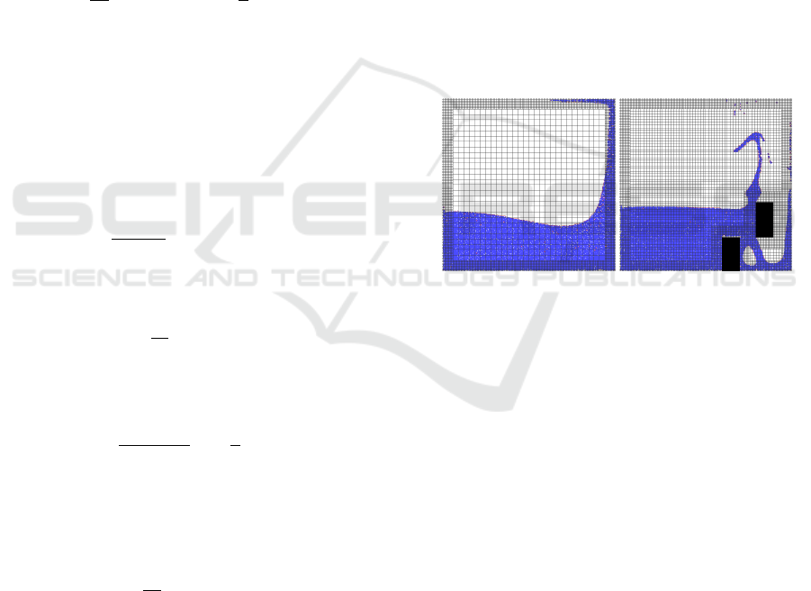
shown in Figure 1.

(a) (b)

Figure 1: The narrow band of ﬁne grid cells can be seen

around all solid boundaries. 1(a) shows the coarse grid with

1 coarse grid cell equal to 16 ﬁne grid cells and narrow band

of ﬁne cells that is 8 ﬁne grid cells wide. 1(b) shows the

coarse grid with 1 coarse grid cell equal to 4 ﬁne grid cells

and narrow band of ﬁne cells that is 8 ﬁne grid cells wide.

Here the narrow band can be seen around the solid obstacles

as well.

Post velocity advection, the Poisson equation is

solved on the coarse and narrow band ﬁne grid us-

ing a preconditioned conjugate gradients solver. Any

other solver of choice can also be used for this step.

If these two grids are used directly to advect the ﬂuid

surface, the coarse grid is not able to resolve the ﬂuid

surface accurately due to its Nyquist limit. This is the

second region where the ﬂuid needs to be accurately

resolved, else all visual details are lost. In order to do

this, the coarse grid has to be upgraded to a ﬁner grid

everywhere in the ﬂuid domain, post the narrow band

pressure solve.

The fundamental idea behind the need for upgra-

dation here is to get velocity on a ﬁner grid every-

where before the ﬂuid surface is advected. This al-

Narrow Band Pressure Computation for Eulerian Fluid Simulation

lows the velocity ﬁeld to have enough degrees of free-

dom to accurately resolve free surface detail. This ve-

locity ﬁeld also has to be divergence free to enforce

mass conservation in the ﬂuid.

We tried two methods for performing the upgrada-

tion. We call these methods upgradation by velocity

interpolation and by pressure ﬁeld smoothing. We de-

scribe both below.

4.1 Upgradation by Velocity

Interpolation

The ﬁrst method upgrades the velocity ﬁeld in the

coarse grid, after the pressure solve. We create a

new ﬁne grid everywhere in the ﬂuid domain. At the

boundary between the coarse and the narrow band ﬁne

grid, velocity is interpolated between the narrow band

values and the coarse grid values from the neighbour-

ing cells and the interpolated value is copied to the

new ﬁne grid. Everywhere else, the value from the

underlying grid (coarse or narrow band ﬁne) is copied

as is. Now, the ﬁnal velocity ﬁeld is available in a ﬁne

grid everywhere in the ﬂuid domain before the liquid

surface is advected and there are enough degrees of

freedom present to compute adequate surface detail.

Algorithm 1 explains what happens in one simulation

step when using this method.

Algorithm 1: Single time step algorithm with velocity ﬁeld

interpolation.

1: Advect u

to u

∗

using Equation 3 on the ﬁne grid

everywhere in the ﬂuid domain.

2: Solve Poisson system given by Equation 4 on the

coarse grid.

3: Solve Poisson system given by Equation 4 on the

narrow band ﬁne grid.

4: Compute velocity u

n+1

on the coarse and narrow

band ﬁne grids using Equation 5.

5: Interpolate the velocity ﬁeld across the coarse and

narrow band ﬁne grid boundary.

6: Copy interpolated velocity to the new ﬁne grid.

7: Extrapolate velocity from the ﬁne grid.

8: Compute the distance ﬁeld φ using Equation 6

and advect the liquid surface.

This method is easy to compute as the interpola-

tion adds minimal overhead to the computation cost.

We, however, found that when the narrow band is

smaller in width than a fourth of the original (i.e., non-

coarse) grid size, the ﬂuid loses mass rapidly, as errors

in the velocity ﬁeld dominate. The maximum speedup

obtained is thus limited when using this upgradation

method. It is also harder to ensure that the ﬁnal up-

graded velocity ﬁeld on the ﬁne grid is divergence

free. Therefore, the method suffers from mass loss

errors.

4.2 Upgradation by Pressure Field

Smoothing

In our next method instead of upgrading the velocity

ﬁeld, we upgrade the pressure ﬁeld itself. In order

to do this, the pressure ﬁeld is interpolated across the

coarse and narrow band ﬁne grid boundary. Then the

pressure ﬁeld is regularized by running 1 − 3 Jacobi

iterations on it. We start by intializing the iteration

using the interpolated pressure ﬁeld on the ﬁne grid

and then solve Equation 4 using the Jacobi iterations.

This ensures that the interpolated ﬁeld is free from

divergence, as is the subsequent velocity ﬁeld com-

puted from it. This is then used to advect the liquid

surface. This method does not suffer from signiﬁcant

mass loss like the velocity interpolation method, and

with careful implementation the Jacobi iteration does

not pose too much of an additional computational bur-

den. Algorithm 2 presents the steps involved in this

method.

The pressure smoothing technique allows us to get

large speedups over a conjugate gradient solve every-

where on a ﬁne grid, without sacriﬁcing the ﬂuid sur-

face details. This makes it very suitable for visual

ﬂuid simulation.

Algorithm 2: Single time step algorithm with pressure ﬁeld

smoothing.

1: Advect u

to u

∗

using Equation 3 on the ﬁne grid

everywhere in the ﬂuid domain.

2: Solve Poisson system given by Equation 4 on the

coarse grid.

3: Solve Poisson system given by Equation 4 on the

narrow band ﬁne grid.

4: Interpolate the pressure ﬁeld across the coarse

and narrow band ﬁne grid boundary.

5: Copy interpolated pressure to the new ﬁne grid.

6: Run upto 3 Jacobi iterations on the pressure ﬁeld

in the ﬁne grid to regularize it.

7: Compute velocity u

n+1

on the ﬁne grid using the

regularized pressure ﬁeld using Equation 5.

8: Extrapolate velocity from the ﬁne grid.

9: Compute the distance ﬁeld φ using Equation 6

and advect the liquid surface.

4.3 Boundary Conditions

There are usually two kinds of boundaries in a free

surface ﬂuid simulation. The boundary between the

ﬂuid and the solid requires a Neumann boundary con-

dition, which is enforced for all cells in the nar-

GRAPP 2017 - International Conference on Computer Graphics Theory and Applications

row band when the narrow band Poisson equation is

solved. The free surface requires a Dirichlet bound-

ary condition, which is carefully enforced for all cells

on the ﬂuid surface during the Poisson solves and

the interpolation done for the pressure ﬁeld smooth-

ing. A third boundary is introduced in the simulation

due to partitioning the ﬂuid domain in coarse and nar-

row band ﬁne cells. Fluid is allowed to move freely

across this boundary so that this boundary appears

completely porous to the ﬂuid during advection.

5 EXPERIMENTAL RESULTS

AND ANALYSIS

We have performed a number of experiments to cat-

alog the efﬁcacy of our methods and also to deter-

mine the kind of errors introduced in the simulation

due to its use. We have performed all our experiments

on a machine with a 16 core Intel 2.60 GHz Xeon

processor with 32 GB of RAM. We solve the Navier-

Stokes by splitting the equations, using operator split-

ting, into advection and pressure projections stages.

The pressure projection step needs to solve a large

linear system at each time step of the simulation. An

incomplete Cholesky preconditioned conjugate gradi-

ent technique is used to solve the voxelized Poisson

equation in this stage (Bridson, 2008). We use this

solver as a base solver in all our simulations. Our

base ﬂuid simulator is parallelized using OpenMP,

with the exception of the preconditioned conjugate

gradient pressure solver, which is implemented seri-

ally. This same solver is used for the Poisson solves

in our narrow band simulator as well.

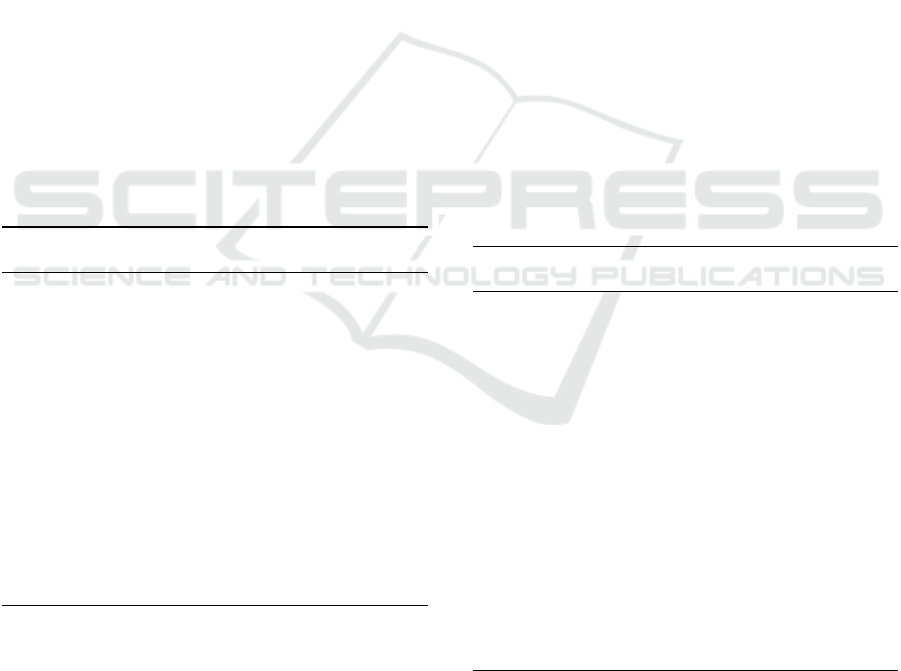
5.1 Performance with Velocity

Interpolation

We applied velocity interpolation based upgradation

(see Section 4.1) to grids with ﬁne narrow bands of

width 64 and 128 cells. Average iteration time, av-

eraged over every 500 frame window, is plotted and

shown in Figure 2 for the narrow band width of 64. It

should be noted that narrow band widths are always

measured in number of ﬁne grid cells. The original

base simulation is a simple dam-break simulation, run

on a 512×512 ﬁne grid. In the coarse grid, the coarse

grid cell size used is double the size of the ﬁne grid

cell size in either dimension. The speedup obtained in

total simulation time is 22.9% and 20.0% for the 64

and 128 sized narrow bands respectively. Reducing

the narrow band grid size below 64 pushes errors in

velocity beyond acceptable limits.

Figure 2: Performance of the ﬂuid simulation when using

the velocity interpolation method with a narrow band of

width 64.

5.2 Performance with Pressure Field

Smoothing

Next, we applied pressure ﬁeld smoothing upgrada-

tion (see Section 4.2) to grids with ﬁne narrow bands

of widths ranging from 8 to 64. The pressure ﬁeld

smoothing method allows much thinner narrow bands

of ﬁne grid cells with less error, thereby offerring

much larger speedups. The original base simulation

is the same as the one used above. Average iteration

time, averaged over every 500 frame window, is plot-

ted and shown in Figure 3. In each case, 3 Jacobi iter-

ations were run to regularize the interpolated pressure

ﬁeld.

Figure 3: Performance of the ﬂuid simulation when using

the pressure ﬁeld smoothing method. Here 1 coarse grid

cell is equal to 4 ﬁne grid cells.

We further pushed the amount of speedup that can

be obtained with our technique by making the coarse

grid cells larger to contain 16 ﬁne grid cells instead

of the earlier 4. The average iteration time is plotted

as before in Figure 4. The speedup obtained in total

simulation time in each case is shown in Table 1. The

second column of the table gives the speedup when 1

coarse grid cell contains 4 ﬁne grid cells, and the third

column when 1 coarse grid cell contains 16 ﬁne grid

cells.

Figure 5 shows a comparison of the per itera-

tion performance of the original simulator with the

Narrow Band Pressure Computation for Eulerian Fluid Simulation

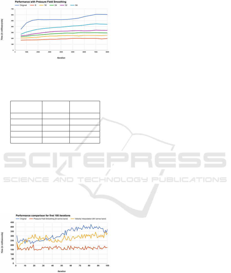
Figure 4: Performance of the ﬂuid simulation when using

the pressure ﬁeld smoothing method with larger coarse grid

cells. Here 1 coarse grid cell is equal to 16 ﬁne grid cells.

Table 1: Percent speedup obtained in total simulation time

over the original base simulation for different narrow band

widths.

Width of Speedup Speedup

narrow band (Coarse 4) (Coarse 16)

8 57.5% 64.4%

16 48.9% 55.1%

24 42.1% 47.7%

32 35.5% 41.5%

64 21.9% 26.8%

fastest velocity smoothing case and the fastest pres-

sure smoothing case, for the ﬁrst 100 iterations of the

simulation. This is comparison of raw per iteration

timing data, without the averaging done in the pre-

vious cases. It can be clearly seen that the pressure

ﬁeld smoothening method gives very large speedups

in comparison to the velocity interpolation method,

for the same original base simulation. We will see

later that is also produces less error in the simulation.

We compare the visual quality of the simulations pro-

duced next.

Figure 5: Comparison of performance of various implemen-

tations of the ﬂuid simulator for ﬁrst 100 iterations.

5.3 Visual Quality Comparison

Figure 6 shows rendered frames from the original 2D

simulator, and the same frames from the simulators

implemented with velocity interpolation and pressure

ﬁeld smoothing at different coarse grid resolutions. It

can be seen that the pressure ﬁeld smoothing results

are visually closer to the original, unaccelerated sim-

ulator. The velocity interpolation method introduces

artefacts in the simulation in the form of additional

air gaps in the ﬂuid volume and also, mass loss. The

size of the narrow band is 64 with velocity interpola-

tion and 8 with pressure ﬁeld smoothing. Between the

two pressure smoothing cases some difference can be

seen, owing to the difference in size of the coarse grid

cells.

We also show some more frames from another

simulation that had additional solid obstacles in the

ﬂuid domain in Figure 7. The narrow band also exists

around the obstacles. It can be seen that our method

correctly resolves all simulation details even around

the obstacles.

Comparison videos of these simulations can be

seen in the supplementary video submitted with the

paper.

5.4 3D Simulation

We performed similar experiments on a 3D ﬂuid sim-

ulator. The methods introduced in this paper work

perfectly in 3D too. The speedup in total simulation

time obtained with pressure ﬁeld smoothing over an

original base dam break simulation on a grid size of

128 × 128 ×128 is 38.0%. This is with a narrow band

size of 24 and with 1 coarse grid cell equal to 8 ﬁne

grid cells. Sample rendered frames of the simulation

can be seen in Figure 8. Visual quality of the results

generated by the pressure ﬁeld smoothed simulator is

comparable to the original unaccelerated simulator.

5.5 Error Analysis

We compute the error introduced in the simulation

due to the approximation introduced by the coarse

grid. We show the difference in velocity in the hor-

izontal and vertical directions in the ﬂuid ﬁeld in Fig-

ure 9, for a single frame. Warmer colors represent

higher error. It can be seen that the velocity interpo-

lation method introduces more error in the ﬂuid than

the pressure smoothing case. Errors also increase as

the coarse grid cell size increases and narrow band

width decreases (see Figure 10). Visual ﬁdelity of

the simulation and error have to balanced against the

speedup obtained during simulation based on compu-

tational requirements and costs.

GRAPP 2017 - International Conference on Computer Graphics Theory and Applications

(a) (b) (c) (d)

(e) (f) (g) (h)

Figure 6: Comparison of visual quality of the simulation produced. 6(a) and 6(e) are two different frames from the original

simulation, 6(b) and 6(f) are the same frames from the simulator implemented with velocity interpolation, 6(c) and 6(g) are

frames from the simulator implemented with pressure ﬁeld smoothing on coarse grid cell size equal to 4, 6(d) and 6(h) are

frames with pressure ﬁeld smoothing on coarse grid cell size equal to 16 ﬁne grid cells.

Figure 7: Comparison of visual quality of the simulation

produced with obstacles in the ﬂuid. The top row shows

frames from the original simulation on a 256 × 256 grid.

The bottom row shows the same frames from the simulator

with pressure ﬁeld smoothing, with 1 coarse grid cell size

equal to 4 ﬁne grid cells and a narrow band of width 8.

Figure 8: Comparison of visual quality of the simulation

produced in 3D. The top row shows frames from the orig-

inal simulation on a 128 × 128 × 128 grid. The bottom

row shows the same frames from the simulator with pres-

sure ﬁeld smoothing on a coarse grid with a narrow band of

width 24.

Narrow Band Pressure Computation for Eulerian Fluid Simulation

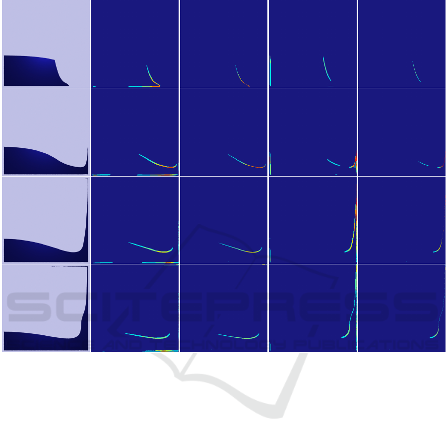
Figure 9: Comparison of error in ﬂuid velocity. The ﬁrst column shows frames 1000, 2000, 3000 and 4000 from the original

simulation, the second and third columns show error in the horizontal component of velocity for velocity interpolation and

pressure smoothing, the fourth and ﬁfth columns show error in vertical component of velocity for velocity interpolation and

pressure smoothing respectively. Blue represents 0 error and red represents maximum error.

6 CONCLUSIONS

We have presented a method to accelerate the pres-

sure projection step in an Eulerian ﬂuid simulator by

solving the Poisson’s equation only in a narrow band

around ﬂuid-solid boundaries. We solve this system

of equations on a coarser grid everywhere else in the

ﬂuid domain and then upgrade this result to a ﬁner

grid to obtain enough degrees of freedom to track

the ﬂuid surface accurately. We present two methods

of performing the upgradation, namely velocity inter-

polation and pressure ﬁeld smoothing. We compare

the pros and cons of each, giving extensive results

about the visual quality of simulations produced, er-

rors introduced in the simulation and the computation

speedup obtained. We conclude that the pressure ﬁeld

smoothing method performs better on all metrics and

is a better way to perform the upgradation than veloc-

ity interpolation. We also show that the same methods

work in a 3D ﬂuid simulator also.

The behaviour of the narrow band computation in

the presence of more complicated, non-grid aligned

obstacles needs more analysis. The role of the size of

the obstacle with respect to the grid size also needs

to be carefully understood. Currently, we have used

a small and conservative timestep size in the narrow

band simulator. We would like to investigate adaptive

timestepping for such simulators as well.

We would like to explore adaptive grid coarsening

during every step of the simulation so that adequate

degrees of freedom are always available at the ﬂuid

surface to resolve detail. This will help us avoid the

grid upgradation step and may lead to better perfor-

mance. We also want to explore the use of our method

GRAPP 2017 - International Conference on Computer Graphics Theory and Applications

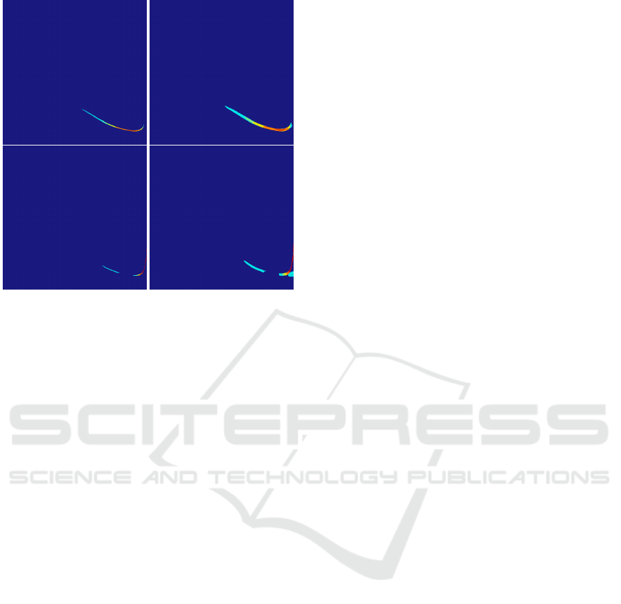
Figure 10: Comparison of error in ﬂuid velocity be-

tween different coarse grid resolutions when using pressure

smoothing. The ﬁrst column shows error in horizontal and

vertical components of velocity when 1 coarse grid cell con-

tains 4 ﬁne grid cells, the second column shows the same

errors when 1 coarse grid cell contains 16 ﬁne grid cells.

The error regions are wider for coarser grids.

in accelerating other ﬂuids simulations such as smoke

and ﬁre.

REFERENCES

Ando, R., Thuerey, N., and Wojtan, C. (2015). A

dimension-reduced pressure solver for liquid simula-

tions. Computer Graphics Forum, 34(2):473–480.

Autodesk. Deep adaptive ﬂuid simulation in Maya 2016.

http://www.autodesk.com/products/maya/features/

dynamics-and-effects/deep-adaptive-ﬂuid-simulation.

Last accessed on 8/6/2016.

Berger, M. and Oliger, J. (1984). Adaptive mesh reﬁnement

for hyperbolic partial differential equations. Journal

of Computational Physics, 53:484–512.

Bridson, R. (2008). Fluid Simulation for Computer Graph-

ics. Taylor & Francis.

Bridson, R., Houriham, J., and Nordenstam, M. (2007).

Curl-noise for procedural ﬂuid ﬂow. ACM Transac-

tions on Graphics, 26(3).

Chentanez, N. and M

uller, M. (2011). Real-time eulerian

water simulation using a restricted tall cell grid. In

ACM Transactions on Graphics, volume 30, page 82.

Chentanez, N., M

uller, M., and Kim, T.-Y. (2014). Coupling

3d eulerian, heightﬁeld and particle methods for in-

teractive simulation of large scale liquid phenomena.

In Proceedings of the ACM SIGGRAPH/Eurographics

SCA, pages 1–10.

De Witt, T., Lessig, C., and Fiume, E. (2012). Fluid simu-

lation using laplacian eigenfunctions. ACM Transac-

tions on Graphics, 31(1):10:1–10:11.

Enright, D., Marschner, S., and Fedkiw, R. (2002). Anima-

tion and rendering of complex water surfaces. ACM

Transactions on Graphics, 21(3):736–744.

Ferstl, F., Ando, R., Wojtan, C., Westermann, R., and

Thuerey, N. (2016). Narrow band FLIP for liquid sim-

ulations. Computer Graphics Forum (Eurographics),

35(2):to appear.

Ferstl, F., Westermann, R., and Dick, C. (2014). Large-scale

liquid simulation on adaptive hexahedral grids. IEEE

Transactions on Visualization and Computer Graph-

ics, 20(10):1407–1417.

Foster, N. and Fedkiw, R. (2001). Practical animation of

liquids. In Proceedings of SIGGRAPH, pages 23–30.

Jung, H. R., Kim, S.-T., Noh, J., and Hong, J.-M. (2013). A

heterogeneous CPUGPU parallel approach to a multi-

grid poisson solver for incompressible ﬂuid simula-

tion. Computer Animation and Virtual Worlds, 24(3-

4):185–193.

Kim, T., Tessendorf, J., and Threy, N. (2013). Closest point

turbulence for liquid surfaces. ACM Transactions on

Graphics, 32(2):15:1–15:13.

Larmorlette, L. and Foster, N. (2002). Structural modeling

of ﬂames for a production environment. ACM Trans-

actions on Graphics, 21(3):729–735.

Lentine, M., Zheng, W., and Fedkiw, R. (2010). A novel al-

gorithm for incompressible ﬂow using only a coarse

grid projection. ACM Transactions on Graphics,

29(4).

Losasso, F., Gibou, F., and Fedkiw, R. (2004). Simulating

water and smoke with an octree data structure. ACM

Transactions on Graphics, 23(3):457–462.

McAdams, A., Sifakis, E., and Teran, J. (2010). A

parallel multigrid poisson solver for ﬂuids simula-

tion on large grids. In Proceedings of ACM SIG-

GRAPH/Eurographics SC, pages 65–74.

Montijn, C., Hundsdorfer, W., and Ebert, U. (2006). An

adaptive grid reﬁnement strategy for the simulation

of negative streamers. Journal of Computational

Physics, 219(2).

Mullen, P., Crane, K., Pavlov, D., Y., T., and Desbrun, M.

(2009). Energy-preserving integrators for ﬂuid anima-

tion. In Proceedings of SIGGRAPH, pages 1–8.

Prakash, A. and Chaudhuri, P. (2015). Comparing per-

formance of parallelizing frameworks for grid-based

ﬂuid simulation on the cpu. In Proceedings of the

8th ACM India Computing Conference, Compute ’15,

pages 1–7.

Rasmussen, N., Nguyen, D., Geiger, W., and Fedkiw, R.

(2003). Smoke simulation for large scale phenomena.

ACM Transactions on Graphics, 22(3):703–707.

Schechter, H. and Bridson, R. (2008). Evolving sub-grid

turbulence for smoke animation. In Proceedings of

the ACM SIGGRAPH/Eurographics SCA, page 17.

Selle, A., Fedkiw, R., Kim, B., Liu, Y., and Rossignac,

J. (2008). An unconditionally stable maccormack

method. Journal of Scientiﬁc Computing, 35(2-

3):350–371.

Stam, J. (1999). Stable ﬂuids. In Proceedings of SIG-

GRAPH, pages 121–128.

Narrow Band Pressure Computation for Eulerian Fluid Simulation

Stomakhin, A., Schroeder, C., Chai, L., Teran, J., and Selle,

A. (2013). A material point method for snow simu-

lation. ACM Transactions on Graphics, 32(4):102:1–

102:10.

Threy, N., Wojtan, C., Gross, M., and Turk, G. (2010).

A multiscale approach to mesh-based surface tension

ﬂows. ACM Transactions on Graphics, 29(4).

Treuille, A., Lewis, A., and Popovi, Z. (2006). Model re-

duction for real-time ﬂuids. ACM Transactions on

Graphics, 25(3):826–834.

Yue, Y., Smith, B., Batty, C., Zheng, C., and Grinspun, E.

(2015). Continuum foam: A material point method for

shear-dependent ﬂows. ACM Transactions on Graph-

ics, 34(5):160:1–160:20.

GRAPP 2017 - International Conference on Computer Graphics Theory and Applications