
Ensemble Kalman Filter based on the Image Structures
Dominique B
´
er
´
eziat
1
, Isabelle Herlin
2
and Yann Lepoittevin
2
1
Sorbonne Universit
´
es, UPMC Univ. Paris 06, CNRS, LIP6 UMR 7606, Paris, France
2
Inria, Paris, France
Keywords:
Domain Decomposition, Ensemble Kalman Filter, Fluid Flows, Localization, Motion Estimation.
Abstract:
One major limitation of the motion estimation methods that are available in the literature concerns the avail-
ability of the uncertainty on the result. This is however assessed by a number of filtering methods, such as the
ensemble Kalman filter (EnKF). The paper consequently discusses the use of a description of the displayed
structures in an ensemble Kalman filter, which is applied for estimating motion on image acquisitions. An
example of such structure is a cloud on meteorological satellite acquisitions. Compared to the Kalman filter,
EnKF does not require propagating in time the error covariance matrix associated to the estimation, resulting
in reduced computational requirements. However, EnKF is also known for exhibiting a shrinking effect when
taking into account the observations on the studied system at the analysis step. Methods are available in the
literature for correcting this shrinking effect, but they do not involve the spatial content of images and more
specifically the structures that are displayed on the images. Two solutions are described and compared in the
paper, which are first a dedicated localization function and second an adaptive domain decomposition. Both
methods proved being well suited for fluid flows images, but only the domain decomposition is suitable for an
operational setting. In the paper, the two methods are applied on synthetic data and on satellite images of the
atmosphere, and the results are displayed and evaluated.
1 INTRODUCTION
The paper describes the use of filtering methods for an
online estimation of motion, associated with its uncer-
tainty measure, on image sequences.
Dense motion estimation approaches originate
from the classic optical flow algorithm (Horn and
Schunk, 1981): the velocity field is computed as the
minimum of an energy function, whose main assump-
tion is the conservation of image brightness on each
point trajectory. This method has been intensively
studied and improved over time and gave birth to a
huge number of papers in the literature. It still faces
the issue of the uncertainty on the result.
Approaches such as the Kalman filter (Kalman,
1960) were introduced in this context for estimating
the uncertainty on the motion result. The Kalman fil-
ter uses an analytical description of the Probability
Density Function associated to the error. It improves
the estimation at each measurement (image acquisi-
tion) as it updates simultaneously the state vector and
its associated covariance matrix. This filter is directly
used in (Elad and Feuer, 1998) on the image bright-
ness values, but with images on size 50 × 50. The
Kalman filter is also applied by (Franke and Rabe,
2005) and (Franke et al., 2005) on the KLT-tracker
features described in (Tomasi and Kanade, 1991). As
the result is a sparse motion field, an extension is de-
fined in (Rabe et al., 2010), where a Kalman filter is
defined for each pixel of the image domain, resulting
in a dense motion estimation. However, as each filter
is defined on a single point, and not on the whole do-
main, it does not include the correlations between two
different pixels of the domain. Defining a global fil-
ter, whose state vector includes a number of variables
for each pixel, is not directly usable for large size im-
ages, due to the huge dimension of the corresponding
covariance matrix (squared number of pixels of the
image) that must be propagated in time.
For operational use, the solution for estimating the
uncertainty on large size systems comes from the en-
semble Kalman filter (EnKF) described in (Evensen,
2003). The approach relies on a sample of the Prob-
ability Density Function associated to the error from
an ensemble of state vectors describing the system.
In case of motion estimation from an image se-
quence, an ensemble of motion and image fields is
designed at initial time, integrated in time and sequen-
140
BÃl’rÃl’ziat D., Herlin I. and Lepoittevin Y.
Ensemble Kalman Filter based on the Image Structures.
DOI: 10.5220/0006096201400150
In Proceedings of the 12th International Joint Conference on Computer Vision, Imaging and Computer Graphics Theory and Applications (VISIGRAPP 2017), pages 140-150
ISBN: 978-989-758-227-1
Copyright
c
2017 by SCITEPRESS – Science and Technology Publications, Lda. All rights reserved

tially improved from the observational image acqui-
sitions. We proposed and described in (Lepoittevin
et al., 2015) the construction of the initial ensem-
ble. A set of state-of-the-art optical flow algorithms
(around 50 methods, described in the surveys (Sun
et al., 2010) and (Baker et al., 2011)) are used to de-
sign the initial ensemble of motion fields. The HS-
brightness method (Sun et al., 2010) is one of these al-
gorithms and it provides the best performance, when
used alone, on our synthetic data. HS-brightness is
a specific implementation of the Horn-Schunk algo-
rithm (Horn and Schunk, 1981), which includes a
multi-resolution scheme and a median filtering (Sun
et al., 2010). Each member of the ensemble is then
integrated in time with the model and an estimate of
motion is computed, at each time, as the average of
the motion members. The uncertainty is described
by the spread of that ensemble. As in (Lepoittevin
et al., 2015) the paper concerns the application of
EnKF for estimating a dense motion field, based on
the structures displayed by images. As the applica-
tion domain concern fluid flows images, we do not
rely on object characteristics, such as the SIFT fea-
tures (Lowe, 1999) and variants, since they are not
significant on these data. The innovation of the paper,
compared to (Lepoittevin et al., 2015), concerns the
use of a segmentation of images by EnKF. Moreover,
we will stress, from the experiments, that merging a
number of optical flow algorithms gives better results
than the best one alone (the HS-brightness method):
all methods take part to the result of EnKF.
Two different alternatives for characterizing the
structures, which are displayed on fluid flows images,
such as fronts and vortices on ocean satellite data, are
compared in the context of EnKF. Comparison con-
cerns two criteria: quality of results and computa-
tional performances.
The first approach, introduced in (Lepoittevin
et al., 2015), concerns the design of a localiza-
tion function that includes information on the dis-
played structures, as it has been discussed for in-
stance in (Anderson, J. L., 2001), (Houtekamer and
Mitchell, 1998), (Hamill et al., 2001), (Oke et al.,
2007) and (Anderson, 2007).
The second approach applies a domain decompo-
sition technique, as in (Nerger et al., 2006) and (Hunt
et al., 2007), which depends on the image brightness
values. This domain decomposition is equivalent to a
segmentation of the image acquisitions.
Both techniques make the estimation depending
on the structures and on their evolution in time.
As the Kalman filter itself is well-known in the
image processing community, Section 2 will shortly
summarize that point and only discuss the mathemat-
ical equations of the ensemble Kalman filter, as ini-
tially given in (Evensen, 2003). Section 3 reminds
about the design of the localization function from im-
age brightness values and its use in the EnKF formal-
ism. The resulting method is named Explicit Struc-
tures Localization in the remaining of the paper. Sec-
tion 4 explains the use of domain decomposition in
the context of EnKF and describes the domain decom-
position associated to a segmentation process. Results
are given in Section 5, which compares the two ap-
proaches. The paper ends with some conclusions and
hints on future research work.
2 EnKF AND EXPLICIT
LOCALIZATION
Let us first provide the notations that are further re-
quired in the paper.
Images are acquired on the spatial domain Ω. A
pixel is denoted p.
A sequence of (N
O
+ 1) acquisitions A
t
,
{
t ∈ [0, N
O
]
}
is processed. An observation vec-
tor Y
t
is computed on each acquisition A
t
. This
vector is either a representation, line by line, of
the image or a description of quantities that are
computing on this image.
A state vector X of size N
X
is defined, whose
value at time t is X
t
= (w
t
, I
t
)
T
. w
t
is the vector de-
scribing the motion field and I
t
is the vector associ-
ated with a synthetic image. The assumption is that
the synthetic image sequence corresponding to I
t
sat-
isfies the optical flow equation: the image brightness
is advected by the motion field.
The objective is to get an estimate X
(a)
t
of the
true state vector (and consequently of the true mo-
tion field), from its background value X
(b)
t
and from
the observation vector Y
t
, so that I
t
is as close as pos-
sible to Y
t
. The background value X
(b)
t
is obtained
from time integration of the estimation X
(a)
t−1
at previ-
ous time.
Ensemble methods rely on a number N
m
of mem-
bers. X
i
t
denotes the state vector at time t of the i
th
member of the ensemble. The average X
t
of the state
vectors X
i
t
is defined by:
X
t
=
1
N
m
N
m
∑
i=1
X
i
t
= X
i
t
(1)
Error terms are discussed in the paper according to the
following notation: E
R
is a centered Gaussian noise
associated to the covariance matrix R and denoted:
E
R
∼ N (0, R) (2)
Ensemble Kalman Filter based on the Image Structures
141

The equations of the Kalman filter (Kalman,
1960) are the following:
1. Let IM be the numerical model describing the
state vector dynamics. Readers should remind
that the studied dynamics is non linear when
studying fluid flows, as advection and convection
processes are involved in the evolution. The back-
ground value X
(b)
t
is obtained from the integra-
tion with IM of the estimation X
(a)
t−1
, computed at
(t − 1):
X
(b)
t
= IMX
(a)
t−1
(3)
The propagation in time of the uncertainty covari-
ance matrix satisfies:
B
(b)
t
= IMB
(a)
t−1
IM
T
(4)
2. If no observation is available at t, the estimation
X
(a)
t
and the matrix B
(a)
t
are taken equal to those
of the background.
3. If an observation vector Y
t
is available at t, the
estimation is computed by:
X
(a)
t
= X
(b)
t
+ K
Y
t
− IHX
(b)
t
(5)
IH is the operator that projects the state vector X
t
in the vector space of Y
t
. K is the Kalman gain,
defined by:
K = B
(b)
t
IH
T
IHB
(b)
t
IH
T
+ R
t
−1
(6)
where R
t
is the covariance matrix associated to the
observation vector. The covariance matrix of the
estimation error is equal to:
B
(a)
t
= B
(b)
t
− KIHB
(b)
t
(7)
The use of EnKF to replace the Kalman filter
comes from an analysis of the computational require-
ments. The Kalman filter requires to store the whole
analytical matrix B
(b)
t
, whose size N
2
X
is usually huge
when processing images: almost 10
7
for a 512 × 512
pixels image with 3 values at each pixel (2 for mo-
tion and 1 for brightness). Moreover, the propagation
in time of this matrix relies on Equation (4), with a
cost N
3
X
. When applying EnKF, an ensemble of state
vectors X
(b),i
t
is defined at each time t and an approx-
imation of the covariance matrix is obtained as:
B
(b)
t
≈ (X
(b),i
t
− X
(b)
t
)(X
(b),i
t
− X
(b)
t
)
T
(8)
with X
(b)
t
=
X
(b),i
t
the average of the ensemble mem-
bers. The whole knowledge available on the system
is then included in the N
m
N
X
matrix containing all
members. The number of members, N
m
, being usu-
ally less than one hundred, the storage cost is drasti-
cally reduced.
Initialized at time 0, the ensemble is integrated
in time by the model IM in Equation (3). If no ob-
servation is available at time t, the estimation X
(a),i
t
is equal to X
(b),i
t
and the uncertainty is approximated
with Equation (8). If an observation Y
t
is available,
X
(a),i
t
is computed according to Equations (5) and (6).
The estimation provided by the ensemble at time t is
calculated as the average of members:
X
(a)
t
= X
(a),i
t
=
1
N
m
N
m
∑
i=1
X
(a),i
t
(9)
Its uncertainty is approximated by replacing
(b)
by
(a)
in Equation (8).
One important remark on the implementation of
EnKF is that all members are involved in the compu-
tation of B
(b)
t
, in Equation (8). Therefore, all members
are included in the computation of the Kalman gain
in Equation (6). Consequently, all members impact
the estimation of member i, which is X
(a),i
t
in Equa-
tion (5). The members are consequently depending
one from the others, when evolving in time. We will
come back to that issue when analyzing results.
EnKF is attractive for both its reduced computa-
tional requirements and its ability to describe the un-
certainty of the result by the members. However, it
also suffers from limitations. One major weakness of
this filter is the approximate knowledge of the back-
ground covariance matrix B
(b)
t
obtained with Equa-
tion (8). This approximation leads to the appearance
of spurious covariance values in the matrix, which im-
pact the quality of the estimation. The next two sec-
tions describe solutions to this limitation, which both
rely on the structures displayed on the fluid flows im-
ages.
3 STRUCTURED EXPLICIT
LOCALIZATION
In this section, we remind the method introduced
in (Lepoittevin et al., 2015). This method is an ex-
plicit localization method. It corrects the background
error covariance matrix B
(b)
t
, in order to recover most
of its analytical properties. For that purpose, the ma-
trix B
(b)
t
is multiplied by a localization matrix ρ before
being used in Equation (6):
L
(b)
t
= ρ ◦ B
(b)
t
(10)
with ◦ the point-wise matrix product.
The matrix L
(b)
t
is then included in place of B
(b)
t
in
the equations that compute the analysis X
(a),i
t
for the
VISAPP 2017 - International Conference on Computer Vision Theory and Applications
142

member i at time t:
X
(a),i
t
= X
(b),i
t
+ K
L
Y(k) − IHX
(b),i
t
(11)
with:
K
L
= L
(b)
t
IH
T
IHL
(b)
t
IH
T
+ R
t
−1
(12)
The values of the matrix ρ are chosen for sup-
pressing the spurious covariances that link pixels,
which should be uncorrelated otherwise. These spu-
rious covariances appear when sampling the error co-
variance matrix and their values decrease if making
use of large size ensembles (but this increases the
computing requirements).
Let p
1
and p
2
denote two pixels of the domain.
The value of their correlation ρ(p
1
, p
2
) depends first
on their distance d
12
= kp
1
− p
2
k (Hamill et al.,
2001). A matrix ρ
d
(the subscript d is the first letter
of distance) is defined with values:
ρ
d
(p
1
, p
2
) =
1 +
d
12
a
d
exp
−
d
12
a
d
(13)
a
d
is a parameter which defines the decorrelation dis-
tance: pixels apart of more than a
d
are no more cor-
related.
The value of ρ(p
1
, p
2
) should also nullify the cor-
relation between the two pixels p
1
and p
2
if they be-
long to different structures. Let I
1
and I
2
denote their
two brightness values and s
12
be equal to |I
1
− I
2
|. A
second matrix ρ
s
is defined:
ρ
s
(p
1
, p
2
) =
1 +
s
12
a
s
exp
−
s
12
a
s
(14)
where a
s
is the decorrelation parameter according to
the brightness similarity between pixels.
The localization function ρ, used in Equation (10),
is then defined as the product of ρ
d
and ρ
s
. Conse-
quently, the correlation values between pixels that are
far apart or belong to different structures are almost
null, as they should have been with the analytical ma-
trix.
The ensemble Kalman filter that is associated to
the localization function ρ is named Explicit Struc-
tures Localization method, or ESL. This filter allows
estimating both a dense motion field (averaging the
members) and its uncertainty, and it relies on the im-
age structures through the matrix ρ. Results obtained
with that filter will be discussed in Section 5 for a di-
rect comparison with those of the method defined in
the next section.
4 DOMAIN DECOMPOSITION
The second approach for limiting the spurious covari-
ances, created by the approximation of B
(b)
t
through
the sampling by an ensemble, is based on a decom-
position of the domain Ω. The decomposition do-
main technique is, for instance, described in (Nerger
et al., 2006), (Hunt et al., 2007) and (Janji
´
c et al.,
2011). The innovation of the paper concerns the use
of the domain decomposition approach for defining
a segmentation of the image acquisitions. A subdo-
main is corresponding to a region of the image. A
dense motion field is then estimated on each subdo-
main with a separate ensemble Kalman filter and the
results are merged on the whole image domain. As
the filters are defined independently on each subdo-
main, the approach imposes that the only non null co-
variances are those between pixels of the same region
(which should correspond to the displayed structures).
The spurious covariances are consequently eliminated
without any numerical process.
We first define the new notations that are required
for describing the method. For simplifying the equa-
tions, the subscript t is suppressed in the following.
The discrete image domain, which includes N
Ω
pix-
els, is decomposed in n
D
subdomains, denoted D
j
for
j = 1, .. ., n
D
. The number of pixels in D
j
is written
N
D
j
. We assume no overlapping between these sub-
domains. Consequently:
N
D
=
n
D
∑
j=1
N
D
j
= N
Ω
(15)
Let us introduce the restriction operator R
D
j
: it re-
stricts any function defined on the image domain as
a function defined on the subdomain D
j
. This allows
defining one EnKF on each subdomain without addi-
tional notation. The merging of the results requires
to define a fusion operator R
D
, which transforms any
function defined on the whole acquisition domain as
a vector composed of the restrictions onto all subdo-
mains. Applying R
D
on any function f , defined on the
image domain leads to the vector f
D
:
R
D
f =
R
D
1
f
.
.
.
R
D
j
f
=
f
D
1
.
.
.
f
D
j
(16)
In the same way, the error covariance matrices
B
(b)
and R are respectively replaced by the merging,
denoted B
(b)
D
and R
D
, of their restrictions on the sub-
domains indexed by j, denoted B
(b)
D
j
and R
D
j
:
B
(b)
D
= R
D
B
(b)
R
T
D
(17)
R
D
= R
D
RR
T
D
(18)
An additional domain decomposition E is de-
signed for the observations. The subdomains of E are
written E
j
, with size N
E
j
. We make use of the same
Ensemble Kalman Filter based on the Image Structures
143

subscript j as each observation subdomain E
j
is asso-
ciated to one estimation subdomain D
j
. The number
of observation subdomains is consequently the same
than the number n
D
of estimation subdomains. In or-
der to allow a continuous (smooth) estimation of mo-
tion, the subdomains E
j
usually overlap, so that the
analysis computed on one pixel p of D
j
uses obser-
vations from all its neighboring pixels, even if p is
located at the boundary of the subdomain D
j
. E
j
is
defined by extending the subdomain D
j
with a given
number of pixels in every direction. The total number
of overlapping pixels N
Ov
is equal to:
N
Ov
= N
E
− N
Ω
(19)
with N
E
=
n
D
∑
j=1
N
E
j
. Let R
E
denote the merging of
the restrictions associated to the observation domain
decomposition E, which is defined similarly to R
D
.
In the following paragraph, we illustrate these
complex notations and we define the quantities B
(b)
D
and B
(b)
E
on a simple example: the image domain is
decomposed into four subdomains, displayed on Fig-
ure 1.
D
1
D
2
D
3
D
4
Figure 1: Decomposition of Ω into four subdomains.
The background error covariance matrix B
(b)
is
first rewritten for expressing the covariances between
pixels belonging to the subdomains D
i
and D
j
:
B
(b)
=
h
B
(b)
D
i, j
i
(20)
Applying the merging of restriction operators, as ex-
plained in Equation(17), gives:
B
(b)
D
=
B
(b)
D
1,1
0 0 0
0 B
(b)
D
2,2
0 0
0 0 B
(b)
D
3,3
0
0 0 0 B
(b)
D
4,4
(21)
The same applies for the observation domain decom-
position by replacing D by E in Equation (21).
Coming back to the general case, an ensemble
Kalman filter is designed on each subdomain D
j
and
makes use of the values of pixels belonging to E
j
. The
filter is based on the following equations:
X
(a),i
= X
(b),i
+ R
D
K
E
R
E
[Y(k) − IHX
(b),i
] (22)
K
E
= B
(b)
E
IH
T
IHB
(b)
E
IH
T
+ R
E
RR
T
E
−1
(23)
Having defined the equations of the Domain De-
composition method, we would like to understand the
links between this method and the Explicit Structures
Localization method, ESL.
Going back to the illustration of Fig 1 and as-
suming no intersection between the observation sub-
domains, we define the observation subdomains by
E
j
= D
j
for each value j. We define the localization
function ρ:
ρ(p
1
, p
2
) =
1 if ∃ j such as p
1
and p
2
∈ D
j
0 otherwise
(24)
The analysis computed by ESL is written for each
member i:
X
(a),i
= X
(b),i
+ K
L
[Y(k) − IHX
(b),i
] (25)
K
L
= L
(b)
IH
T
IHL
(b)
IH
T
+ R
−1
(26)
with
L
(b)
= ρ ◦ B
(b)
(27)
It must be compared with the analysis of DD com-
puted from Equations (22) and (23). As E = D, these
two last equations are simplified:
X
(a),i
= X
(b),i
+ R
D
K
D
R
D
[Y(k) − IHX
(b),i
] (28)
K
D
= B
(b)
D
IH
T
IHB
(b)
D
IH
T
+ R
D
RR
T
D
−1
(29)
If R is additionally supposed diagonal, Equation (29)
is rewritten as:
K
D
= B
(b)
D
IH
T
IHB
(b)
D
IH
T
+ R
−1
(30)
The multiplication, in Equation (27), of B
(b)
by
the function ρ, defined in Equation (24), results in a
block diagonal matrix. Each block is associated to
a subdomain D
j
. L
(b)
is then equal to B
(b)
D
of Equa-
tion (21). Therefore, the two Kalman gains, K
D
from
Equation (30) and K
L
from Equation (26), are equal
and the two analysis values, defined by Equations (28)
and (25), are the same. DD and ESL are equivalent in
this simple setting.
The Domain Decomposition approach shows
however major computational advantages compared
to the Explicit Structures Localization. The Reader
should first notice that B
(b)
D
is a block diagonal matrix
and we remind that R is taken as diagonal in most ap-
plications. Therefore, the matrix to be inverted when
computing the Kalman gain in Equation (23) is block
diagonal. Its inverse is composed of the inverses
VISAPP 2017 - International Conference on Computer Vision Theory and Applications
144

of each block, which may be computed by indepen-
dent processors in a parallel implementation. The
computational cost of the matrix inversion, required
when computing the Explicit Structures Localization
method, is equal to N
Ω
3
, while the Domain Decom-
position only requires (
∑
n
D
j=1
N
D
3
j
) computations, with
the property:
N
Ω
3
=
n
D
∑
j=1
N
D
j
!
3
(
n
D
∑
j=1
N
D
3
j
) (31)
The overlapping of the observation subdomains
is mandatory for avoiding discontinuities in the re-
sult. Otherwise, two pixels p
1
and p
2
, located on
both sides of the boundary between neighboring sub-
domains, would be totally uncorrelated. This is illus-
trated by Figure 2, which is the result of motion esti-
mation obtained without overlapping the observation
subdomains. The zoom displayed on the right image
illustrates the discontinuity at the boundary between
two subdomains.
Figure 2: Left to right: Motion background w
(b)
; Motion
estimation w
(a)
; Highlight on discontinuities between sub-
domains.
If the observation subdomains are overlapping, the
Kalman gain, in Equation (23), is computed for each
subdomain E
j
. But the value of the estimation X
(a),i
is only updated for pixels belonging to the estimation
subdomain D
j
. Two neighboring pixels p
1
and p
2
, lo-
cated on both sides of the two neighboring domains
D
j
1
and D
j
2
, are updated by computations performed,
respectively, on the two observation domains E
j
1
and
E
j
2
. If E
j
1
and E
j
2
overlap, p
2
belongs to E
j
1
. When
the Kalman gain is computed for pixel p
1
, it includes
the covariance between p
1
and pixels of E
j
1
, and con-
sequently pixel p
2
. This makes the result smoother
and more significant at the boundary between the sub-
domains.
Unfortunately, the overlapping of observation
subdomains also results in additional computations,
as the Kalman gain is computed several times for the
pixels belonging to the intersection between subdo-
mains. Let N
D
Max
denote the number of pixels of
the largest subdomain D
Max
and N
E
Max
the number
of pixels in the corresponding observation subdomain
E
Max
. The additional computation cost for each sub-
domain is bounded by the number of pixels included
in the region E
Max
− D
Max
, which is supposed to be
low compared to N
D
Max
. As n
D
processors compute
simultaneously the Kalman gain in the n
D
observation
subdomains, the total cost of computing the Kalman
gain is a function of N
E
3
Max
, which is approximately
equal to N
D
3
Max
, according to the previous assump-
tion. This value has to be compared with the com-
plexity O(N
Ω
3
) of the Explicit Structures Localiza-
tion, with N
Ω
N
D
Max
. The Domain Decomposition
therefore becomes an affordable approach for estimat-
ing motion with EnKF in an operational setting, as the
size of the largest region may be defined according to
the computational constraints.
The Domain Decomposition is usually applied, as
described by Hunt et al. (Hunt et al., 2007), accord-
ing to regular grids. The subdomains are rectangles,
whose dimensions correspond to an empirical estima-
tion of the decorrelation value. However, the decom-
position in subdomains should rely on the structures
displayed on images, so that the covariances become
negligible for pixels belonging to different structures.
The decomposition proposed in our paper relies on
a split-and-merge approach, which is a segmentation
technique that has been widely used for image pro-
cessing (the Reader may refer to the foundational pa-
per of Horowitz and Pavlidis (Horowitz and Pavlidis,
1976)). The split-and-merge segmentation is based
on a quadtree partition of the image. Starting from
the whole image, the splitting is iterated as long as
each new region is heterogeneous. A merging phase is
then applied, in which regions with similar properties
are combined. The merging phase aims to reduce the
number n
D
of subdomains. An extended observation
subdomain E
i
is then associated to each subdomain D
i
in order to impose the smoothness property, as it has
been previously justified. Having minimized the num-
ber n
D
of subdomains consequently minimizes the
number N
Ov
of overlapping pixels in the observations
subdomains. The parameters involved in the split-
and-merge method are related to the distance and the
similarity between pixels. The first parameter defines
the maximal size of an analysis subdomain D
j
. If we
want to compare the domain decomposition method
to the ESL technique, this maximal size is chosen so
that the distance between two pixels belonging to D
j
is lower than the decorrelation value used with the
ESL approach. The second parameter defines the no-
tion of homogeneous region. In other words, it de-
fines which properties should be verified by the pixels
of an analysis subdomain D
j
, so that D
j
is considered
as homogeneous. The classical choice is to consider
that the standard deviation σ
j
of the gray level val-
ues within the subdomain D
j
should be smaller than
a given threshold. In order to compare with the ESL
Ensemble Kalman Filter based on the Image Structures
145
method, the value of σ
j
is chosen to be equal to the
brightness decorrelation value of ESL.
5 DESCRIPTION OF THE
EXPERIMENTS
This section displays and discusses results obtained
with both the ESL and DD approaches, but we remind
that only DD is also applied in an operational setting
as the computation is done in parallel for each sub-
domain. The two methods are set up with the same
criteria on the size of regions and on the similarity of
gray level values, in order to get an objective compar-
ison of results with the same modeling of structures.
A last component has to be defined which is the
model of dynamics IM used in Equation (4). In our
experiments, this model assume the Lagrangian con-
stancy of velocity on each pixel trajectory and the
transport of the image brightness by velocity:
∂w
∂t
(x,t) + (w.∇)w(x,t) = 0 (32)
∂I
∂t
(x,t) + w.∇I(x,t) = 0 (33)
The next subsections discuss first the results on
synthetic data and then demonstrate its properties on
satellite acquisitions.
5.1 Synthetic Experiment
The first experiment relies on a sequence of 9 syn-
thetic images, which have characteristics similar to
satellite acquisitions. These images are obtained
by integrating in time, with the model IM of Equa-
tions (32) and (33), the motion field displayed on top
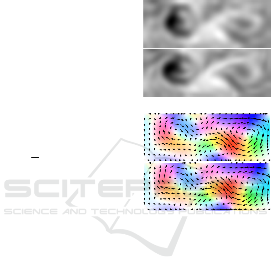
of Figure 4 and the satellite image on top of Figure 3.
This process allows, not only to obtain the sequence
of image observations used for testing motion estima-
tion methods, but also to compute the ground truth on
motion. The bottom parts of the two previous Figures
display the last image of the sequence and the ground
truth on motion at the corresponding time.
In the following, we discuss the results obtained
with our two methods, ESL and DD, and compare
with those of the HS-brightness algorithm (Sun et al.,
2010), which gets the best performances among all
methods, which have been tested on our experimental
data.
Figure 5 provide the results that are computed at
the beginning of the sequence, while Figure 6 illus-
trates the results obtained at the last time. It should be
noted that, in the first case, HS-brightness estimates
Figure 3: First and last image of the synthetic sequence.
Figure 4: Ground truth on motion.
motion from images 1 and 2, while in the second case
this is between images 8 and 9.
Figure 7 displays the domain decomposition that
is used for the DD approach, which is regular in that
experiment.
The motion estimation obtained with the three
methods are visually equivalent and close from the
ground truth displayed on Figure 4. For an improved
understanding of the methods, we computed statis-
tics on the errors of the estimations with regard to
the ground truth. At initial time, the angular errors
of the three methods ESL, DD and HS-brightness are
approximately the same and around 9 degrees. How-
ever, at the last time, the angular errors of the three
methods are different and respectively of 9.0, 9.6 and
10.33 degrees for ESL, DD and HS-brightness. HS-
brightness is one of the initial member of the ensem-
ble and it has demonstrated to be the best member.
However, the other members are contributing during
time integration to that member as we previously dis-
cussed. At the last time, ESL and DD perform better
than their best member. That means that all meth-
VISAPP 2017 - International Conference on Computer Vision Theory and Applications
146
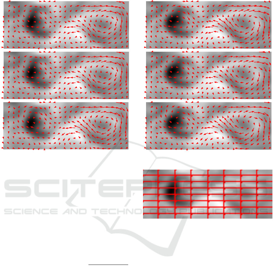
Figure 5: Result of ESL (top), DD (bottom) and HS-
brightness (bottom) on the first image.
ods are contributing in the results. Apart of the result
quality, the main advantage of DD compared to ESL
concerns the computational time, which is divided by
the number of subdomains, which is 64 for this illus-
tration.
One additional output of the ESL and DD meth-
ods, compared to HS-brightness, is the uncertainty
of the motion estimation, as discussed in Sections 3
and 4. We first design an image of the uncertainty on
the orientation of motion at each time t. Let w
i
e
(x,t)
be the value of the i
th
member, at location x and
time t, and w
e
(x,t) be the estimation of the ensem-
ble Kalman filter, obtained as the average of all mem-
bers values. We define U (x,t) =
\
w
i
e
(x,t), w
e
(x,t).
This is the average of the angular difference between
each member i and the estimation. This character-
izes the angular spread of the ensemble at pixel x
and time t. We also compute the map of angular er-
rors, E(x,t) =
\
w
GT
(x,t), w
e
(x,t), between the ground
truth w
GT
(x,t) and the estimation w
e
(x,t). This pro-
cess is illustrated on Figures 8 and 9 where the two
images U(x,t) and E(x,t), computed for the method
DD at the first and last time of the sequence, are dis-
played. Results are similar with the method ESL. It
is visible that the uncertainty measured by the ensem-
ble is linked to the error of the estimation. Further
analysis is part of the perspectives of this research.
Having analyzed the results on synthetic data, we
will demonstrate the potentiality of ESL and DD on
Figure 6: Result of ESL (top), DD (middle) and HS-
brightness (bottom) on the last image.
Figure 7: Domain decomposition.
satellite acquisitions, in the next subsection.
5.2 Satellite Data
Experiments were further conducted with meteoro-
logical satellite sequences, such as the one displayed
on Figure 10 (frames 1, 4, 8, 11, 15, 18).
The domain decomposition obtained with the
split-and-merge algorithm is given on Figure 11. This
gives a rough segmentation on the image, as the
boundaries of the clouds structures are not accurately
defined.
Motion results obtained with the ESL, DD and
HS-brightness methods are visualized on Figure 12
for the initial time and Figure 13 for the last time.
Motion results of ESL and DD are equivalent, but
the computational time required by DD is 55 less than
the one of ESL, since the split-and-merge divides the
whole domain in 55 subdomains. Results of HS-
brightness show that this approach is less suited on
the real satellite data. As HS-brightness is the best of
Ensemble Kalman Filter based on the Image Structures
147
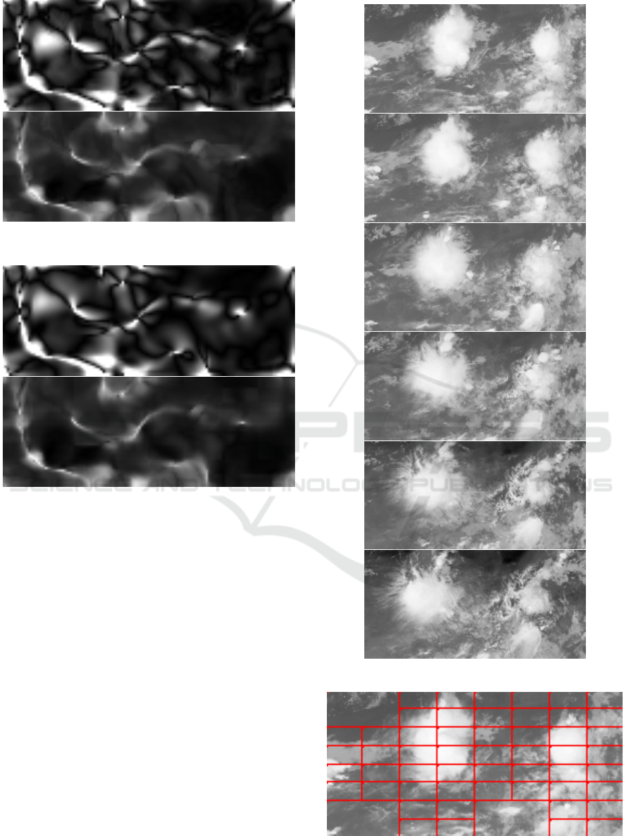
Figure 8: Angular error map of DD, E
DD
, (top) and uncer-
tainty of angular error of DD, U
DD
, on the first image.
Figure 9: Angular error E(x) and uncertainty on the orien-
tation U (x), with DD at last time.
the 50 members used in the two methods, this also
demonstrates again that EnKF makes use of all its
members and that all methods are contributing to the
final estimation.
Figure 14 shows the uncertainty map, previously
named image U(x), computed for the DD method at
the first time.
6 CONCLUSIONS
This paper describes the design of an ensemble
Kalman filter that estimates motion on fluid flows im-
ages and provides a measure on the uncertainty of
the result. For suppressing the spurious covariances,
coming from the sampling of the PDF by an ensem-
ble, two methods are compared which rely on the
structures displayed on the data. On the one hand, the
Explicit Structures Localization method, ESL, which
was defined in the past by the authors, makes use of
a localization function for keeping correlated the only
Figure 10: Six satellite acquisitions.
Figure 11: Domain decomposition performed by DD on the
first observation.
VISAPP 2017 - International Conference on Computer Vision Theory and Applications
148
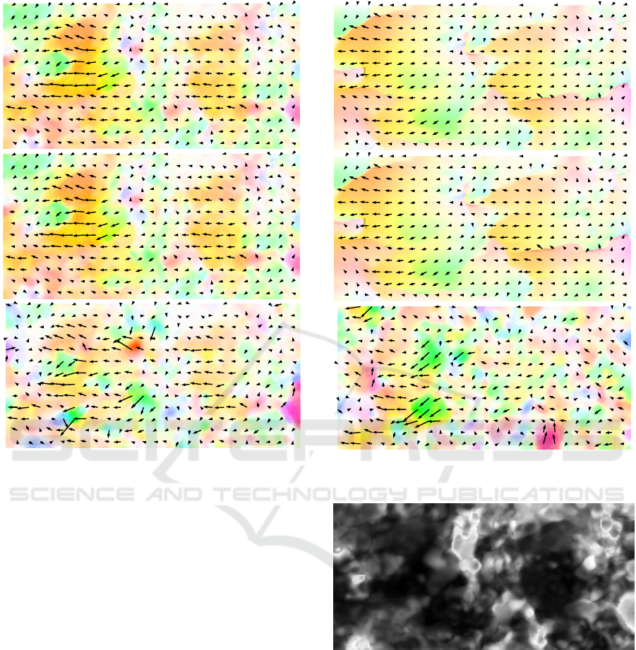
Figure 12: Comparison of ESL (top), DD (middle) and HS-
brightness (bottom) at initial time.
pixels, which are simultaneously close (distance prop-
erty) and having similar gray level values (brightness
property). On the other hand, the innovation of the
paper concerns a Domain Decomposition approach,
named DD, which is based on a rough segmentation
of the image and allows processing each subdomain
in parallel. The two methods have been proven to be
equivalent on synthetic and satellite data, but only the
Domain Decomposition approach is applicable in an
operational setting, due to its reduced computational
requirements.
Various perspectives are considered for this re-
search. First, an improved space-time decomposi-
tion of the domain will be implemented as this is the
key point for both decreasing the number of subdo-
mains (and decreasing the computational cost), while
correctly characterizing the structures. On a method-
ological point of view, the research will consider ap-
proaches such as LETKF (Local Ensemble Transform
Kalman Filter, see (Miyoshi et al., 2007)) for improv-
ing the estimation of the uncertainty computed from
the ensemble. Last, the use of the uncertainty for op-
erational applications such as rain quantity forecast
will be further assessed.
Figure 13: Comparison of ESL (top), DD (middle) and HS-
brightness (bottom) at last time.
Figure 14: Uncertainty computed by DD at first time.
REFERENCES
Anderson, J. L. (2007). An adaptive covariance inflation
error correction algorithm for ensemble filters. Tellus
Series A : Dynamic meteorology and oceanography,
59:210–224.
Anderson, J. L. (2001). An Ensemble Adjustment Kalman
Filter for Data Assimilation. Monthly Weather Re-
view, 129(12):2884–2903.
Baker, S., Scharstein, D., Lewis, J. P., Roth, S., Black, M. J.,
and Szeliski, R. (2011). A database and evaluation
Ensemble Kalman Filter based on the Image Structures
149

methodology for optical flow. International Journal
on Computer Vision, 92(1):1–31.
Elad, M. and Feuer, A. (1998). Recursive optical flow esti-
mation – adaptive filtering approach. Journal of Visual
Communication and Image Representation, 9(2):199–
138.
Evensen, G. (2003). The ensemble Kalman filter: Theoret-
ical formulation and practical implementation. Ocean
Dynamics, 53:343–367.
Franke, U. and Rabe, C. (2005). Kalman filter based depth
from motion with fast convergence. In Intelligent Ve-
hicles Symposium.
Franke, U., Rabe, C., Badino, H., and Gehrig, S. (2005).
6d-vision: Fusion of stereo and motion for robust en-
vironment perception. In DAGM Symposium.
Hamill, T. M., Whitaker, J. S., and Snyder, C. (2001).
Distance-dependent filtering of background error co-
variance estimates in an ensemble Kalman filter.
Monthly Weather Review, 129:2776–2790.
Horn, B. and Schunk, B. (1981). Determining optical flow.
Artificial Intelligence, 17:185–203.
Horowitz, S. L. and Pavlidis, T. (1976). Picture segmen-
tation by a tree traversal algorithm. Journal ACM,
23(2):368–388.
Houtekamer, P. L. and Mitchell, H. L. (1998). A sequential
ensemble Kalman filter for atmospheric data assimila-
tion. Monthly Weather Review, 129:123–137.
Hunt, B. R., Kostelich, E. J., and Szunyogh, I. (2007). Ef-
ficient data assimilation for spatiotemporal chaos: A
local ensemble transform Kalman filter. Physica D:
Nonlinear Phenomena, 230(1):112–126.
Janji
´
c, T., Nerger, L., Albertella, A., Schr
¨
oter, J., and
Skachko, S. (2011). On domain localization in
ensemble-based Kalman filter algorithms. Monthly
Weather Review, 139(7):2046–2060.
Kalman, R. E. (1960). A new approach to linear filtering
and prediction problems. Transactions of the ASME–
Journal of Basic Engineering, 82(Series D):35–45.
Lepoittevin, Y., Herlin, I., and B
´
er
´
eziat, D. (2015). An
image-based ensemble kalman filter for motion esti-
mation. In International Conference on Computer Vi-
sion Theory and Applications.
Lowe, D. (1999). Object recognition from local scale-
invariant features. In International Conference on
Computer Vision.
Miyoshi, T., Yamane, S., and Enomoto, T. (2007). Localiz-
ing the error covariance by physical distances within
a local ensemble transform Kalman filter (LETKF).
Scientific Online Letters on the Atmosphere, 3:8992.
Nerger, L., Danilov, S., Hiller, W., and Schr
¨
oter, J. (2006).
Using sea-level data to constrain a finite-element
primitive-equation ocean model with a local SEIK fil-
ter. Ocean Dynamics, 56(5-6):634–649.
Oke, P. R., Sakov, P., and Corney, S. P. (2007). Impacts of
localisation in the EnKF and EnOI: experiments with
a small model. Ocean Dynamics, 57(1):32–45.
Rabe, C., Mller, T., Wedel, A., and Franke, U. (2010).
Dense, robust, and accurate motion field estimation
from stereo image sequences in real-time. In Euro-
pean Conference on Computer Vision.
Sun, D., Roth, S., and Black, M. (2010). Secrets of opti-
cal flow estimation and their principles. In European
Conference on Computer Vision, pages 2432–2439.
Tomasi, C. and Kanade, T. (1991). Detection and tracking
of point features. Technical Report CMU-CS-91-132,
Carngie Mellon University.
VISAPP 2017 - International Conference on Computer Vision Theory and Applications
150
