Measuring Human-made Corner Structures with a

Robotic Total Station using Support Points, Lines and Planes

Christoph Klug, Dieter Schmalstieg and Clemens Arth

Institute for Computer Graphics and Vision, Graz University of Technology,

Inffeldgasse 16/II, 8010 Graz, Austria

Keywords:

Robotic Total Station, Reﬂectorless Electrical Distance Measurement.

Abstract:

Measuring non-planar targets with a total station in reﬂectorless mode is a challenging and error-prone task.

Any accurate 3D point measurement requires a fully reﬂected laser beam of the electronic distance meter and

proper orientation of the pan-tilt unit. Prominent structures like corners and edges often cannot fulﬁll these

requirements and cannot be measured reliably.

We present three algorithms and user interfaces for simple and efﬁcient construction-side measurement cor-

rections of the systematic error, using additional measurements close to the non-measurable target. Post-

processing of single-point measurements is not required with our methods, and our experiments prove that

using a 3D point, a 3D line or a 3D plane support can lower the systematic error by almost a order of magni-

tude.

1 INTRODUCTION

Total stations are commonly used for measuring an-

gles, distances and 3D points in surveying and build-

ing construction (Uren, 2010). A robotic total sta-

tion, which can be remotely controlled, is equipped

with an electronic distance meter (EDM), which uses

a laser signal for accurate distance measurements

The simpliﬁed and calibrated geometric model of a

common robotic total station without parallax effects

between EDM and camera is shown in Fig. 1. In

the ideal case, all coordinate systems are perfectly

aligned: The EDM is aligned with the principal ray

of the camera; the local spherical coordinate system

of the instrument is aligned with the camera coordi-

nate system, and the camera center is at the origin of

the instrument coordinate system. Adjustment screws

on the device allows an approximation of the ideal

model, but for accurate measurements, an extended

geometric model and device calibration is necessary.

Such calibration includes camera parameters, temper-

ature compensation and EDM corrections

Details about EDM types can be found in (Amann

et al., 2001).

Details about extended geometric models, environmen-

tal inﬂuences and calibrations of total stations can be found

in (Schulz, 2007; Uren, 2010; Nichols and Beavers, 2003;

Coaker, 2009; Reda and Bedada, 2012; Martin and Gatta,

2006).

vertical angle 

(D, , )

horizontal angle 

cam

EDM

instr

(zenith)

inst

instr

img

EDM

principal point

(, )

cam

EDM distance D

Figure 1: Simpliﬁed geometric model for a calibrated

robotic total station with azimuth angle θ, polar angle φ

and radial distance D. In this simpliﬁed version the coor-

dinate system of the EDM is aligned with the camera co-

ordinate system as well as the spherical coordinate frame

robotic total station. Real-world devices require six degrees

of freedom (DOFs) pose conversations between the coordi-

nate frames as well as further corrections.

For standard measurements, reﬂective measurement

targets with known calibration parameters are used.

Modern total stations also support reﬂectorless mea-

surements using the diffuse reﬂection of natural sur-

faces. This is often referred to as measuring nat-

ural targets. Common natural targets in surveying

and building construction should have a high recall

value, thus, preferred targets are corners and edges

of human-made structures. Inﬂuences of the laser

Klug C., Schmalstieg D. and Arth C.

Measuring Human-made Corner Structures with a Robotic Total Station using Support Points, Lines and Planes.

DOI: 10.5220/0006096800170027

In Proceedings of the 12th International Joint Conference on Computer Vision, Imaging and Computer Graphics Theory and Applications (VISIGRAPP 2017), pages 17-27

ISBN: 978-989-758-227-1

EDM

Projected laser dot

Figure 2: For a common refectorless measurement target

with one visible approximately planar surface, the laser dot

must be fully reﬂected by the surface to get reliable distance

results, precluding direct targeting of the corner. The mini-

mum vertical and horizontal measurement error e is approx-

imately deﬁned by e = d

+ r

, where d

is the safety dis-

tance between the edges of the target and the laser pointer,

and r

is the radius of the projected laser beam (approx-

imating the elliptical projection of the laser through a cir-

cle). d

is inﬂuenced by user experience, image resolution,

focal length of the camera, image blur due to out-of-focus

problems, back light conditions and other effects.

beam divergence of the EDM, angular resolution of

the theodolite, inaccurate targeting and optical limi-

tations are reasons why direct measurements of non-

planar targets are critical and error-prone tasks. Sur-

veyors often use post-processing methods to increase

the accuracy of such measurements.

The wide variety of measurement conditions, the

demanding requirements for the results of the mea-

surement procedure regarding accuracy and reliabil-

ity, and the aim to perform single-view metrology

(Criminisi et al., 2000; Hartley and Zisserman, 2003)

make multi-view photogrammetric algorithms largely

inapplicable in realistic scenarios. Practical applica-

tions in indoor and outdoor environments can suf-

fer from problems caused by sunlight and strong

back-light, shadows, large distance measurements

and partly occluded targets. All these issues are not

fully solved problems in Computer Vision in general

per se. Eventually the absence of multiple measure-

ments and observations from multiple camera poses

prohibits the usage of classic photogrammetry algo-

rithms as such.

In this work, we therefore address the problem of

reﬂectorless measuring targets with at least one quasi-

planar surface visible to the total station (see Fig. 2),

using three different methods. Post-processing and

high density 3D point cloud scans are avoided to keep

the measurement effort as low as possible. Since the

projected laser dot should be fully located within the

planar surface to avoid distance measurement errors,

a systematic angular and distance error occurs, which

depends on the projected laser dot size, the observa-

tion angle of the surface and other parameters

. With

See Juretzko (Juretzko, 2004) for an extensive discus-

our algorithms, it is possible to reduce the systematic

measurement error by applying image-based correc-

tions directly in the ﬁeld. As a side effect, the ap-

proach proposed simpliﬁes the overall measurement

procedure, such that even non-experts in the ﬁeld can

perform reliable and robust measurements. This is

proven by the results of our pilot study.

2 RELATED WORK

In the following, we shortly review related work about

using total stations for measuring.

The book by Uren (Uren, 2010) provides an ex-

tensive description of GPS measurements, total sta-

tions and laser range meters, explaining basic survey-

ing and measurement methods, surveying hardware,

software and tools, possible sources of errors and er-

ror propagations. Image-based measurement correc-

tions are not described, however. Coaker (Coaker,

2009) investigated accuracy, precision and reliabil-

ity of reﬂectorless total station measurement methods,

also mentioning the problem of direct measurements

of corners and edges. Similarly, Zeiske (Zeiske, 2004)

describes basic surveying methods and ofﬂine correc-

tions for 2D corner measurements using simple ge-

ometry. However, no online method or image-based

geometric correction are mentioned.

Many modern total stations are already equipped

with image-based measurement methods, like steer-

ing the total station to selected pixels, selecting and

visualizing 3D targets in the image or visualizing

metadata. Scherer et al. (Scherer, 2001; Scherer and

Lerma, 2009) investigated possible beneﬁts of image-

based features for architectural surveying. The de-

vice of Topcon (Topcon Corporation, 2011) supports

an image-based measurement feature for not directly

measurable targets like corners and edges, but with-

out providing any mathematical details or evaluation

of the methods.

Ehrhart et al. (Ehrhart and Lienhart, 2015) investi-

gate image processing methods for deformation mon-

itoring. In their work they detect movements of com-

plete regions by comparing image patches acquired

with the camera of a total station, however, without

explicitly performing any structural analysis of build-

ing corners or edges.

Siu et al. (Siu et al., 2013) describe a close range

photogrammetric solution for 3D reconstruction and

target tracking by combining several total stations and

cameras. Jadidi et al. (Jadidi et al., 2015) use im-

age based modelling to reconstruct 3D point clouds

sion of this problem.

VISAPP 2017 - International Conference on Computer Vision Theory and Applications

and register as-built data to as-planned data. Fathi et

al. (Fathi and Brilakis, 2013) generate 3D wire dia-

grams of a roof using video streams from a calibrated

stereo camera set. Their algorithm combines feature

point matching, line detection and a priori knowledge

of roof structures to a structure from motion pipeline.

Even if the results of these approaches are quite im-

pressive, none of them can be applied for measur-

ing corner and edge structures from a single position.

Fathi et al. further notes accuracy problems of the re-

constructed models.

Closely related to our approach is the work by Ju-

retzko (Juretzko, 2004), who provides conceptional

descriptions for not directly measurable target using

intersections of 3D rays, lines and planes. How-

ever, no comparative study between the methods,

no detailed mathematical description and no suitable

user interface is provided. Furthermore, the author

mentions only minimal measured point sets for each

method without any model ﬁtting approach.

To the best of our knowledge, we are the ﬁrst to

proper describe such measurement techniques with

a detailed mathematical formalism, together with a

comparative study. Moreover we are the ﬁrst to in-

vestigate the measurement concept in detail in an out-

door scenario, giving results and insights into the is-

sues arising outside of laboratory conditions in a prac-

tical working environment.

3 TEST HARDWARE AND

LIMITATIONS

The total station we used for our experiments (see

Fig. 3) had been fully calibrated by the manufacturer.

It provides a closed source driver for controlling the

device, for retrieving the camera image and for trans-

lating between all coordinate systems. As common

for commercially available systems, there is no direct

access to the raw data of the sensors, the geometric

model and the related parameters. The applied cor-

rection algorithms are conﬁdential and kept secret by

manufacturers. While in our case the available API

does not provide a projection matrix, it offers a com-

plete API for coordinate system conversions. There-

fore, we use the simpliﬁed geometric model, which is

shown in Fig. 1, for a calibrated robotic total station

to explain our methods.

Note that whether or not it is theoretically pos-

sible to perform full manual calibration for a single

instance of a device at hand, it is neither reasonable

to assume that every device is shipped with a calibra-

tion by the manufacturer that is perfect for each possi-

ble measurement situation, nor is manual calibration

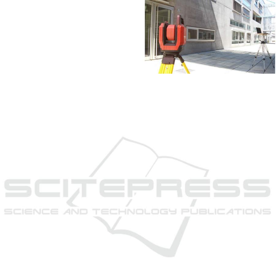
Figure 3: Robotic Total Station and mobile PC used in our

experiments. The communication between the devices is

done wirelessly over WLAN.

easily possible given the level of access provided by

APIs. Thus our assumption to work with the stock

calibrated device as is and employing our simpliﬁed

geometric model is plausible.

4 CONCEPT

We use the standard single point measurement

method as reference method and deﬁne three new

measurement methods, which integrate in-the-ﬁeld

corrections for corner and edge measurements:

(a) Direct reﬂectorless target measurement

(b) Reﬂectorless target measurement using a support

point

line

(d) Reﬂectorless target measurement using a support

plane

Figure 4 shows the direct measurement method as

well as the support point, support line and support

plane method. Details about the methods are provided

in following sections.

4.1 Standard Method

When measuring a corner directly in reﬂectorless

mode, the laser dot must be fully reﬂected by an at-

tached surface. Fig. 1 shows the simpliﬁed geometric

model for a single point measurement, while Fig. 2

shows the systematic error introduced by the afore-

mentioned constraint.

Measurement Flow. The simple measurement ﬂow

is deﬁned by following steps:

1. Use the pan/tilt control interface, until the target-

of-interest is visible in the image

2. Deﬁne target-of-interest in the image

Measuring Human-made Corner Structures with a Robotic Total Station using Support Points, Lines and Planes

)

Figure 4: Four different measurement methods of a cor-

ner with a single visible adjacent area: direct method (a),

support point method (b), support line method (c), support

plane method (d). The numbers in the image indicate the

minimum measurement count and the respective order used

in our algorithms.

3. Calculate the 3D position of the target-of-interest

by measuring the angle and distance at the se-

lected image point

Calculating the Point. A total station deﬁnes a lo-

cal spherical coordinate system. A point is deﬁned by

the horizontal angle ϕ, the vertical angle θ and the

distance D. The simpliﬁed relation between spherical

and Euclidean coordinates for our test device is given

by following equations:

F(x, y, z) =















+ y

+ z

arctan





= atan2(x, y)

arccos



√









(1)

with

D ≥ 0 −π ≤ θ < π 0 ≤ ϕ < π (2)

Note that the azimuth angle ϕ is measured clockwise

and is related to the Cartesian y direction rather than

counterclockwise and related to to the Cartesian x di-

rection. This leads to swapped x and y variables in the

expression atan2(x, y) in Eqn. 1.

The inverse operation can be generalized to a 3D Eu-

clidean rotation for a right-handed coordinate system:

Q(θ, ϕ) = R

(−θ) ·R

(0) ·R

(−ϕ) (3)

p =





= G(D, θ , ϕ) = Q(θ , ϕ) ·





(4)

where p describes a 3D point in Euclidean coordi-

nates and (D, θ , ϕ) describes a 3D point in spherical

coordinates; R

, R

are 3D rotation matrices in

the Euclidean right-handed coordinate system around

the x-axis, y-axis and z-axis, respectively. Q(θ, ϕ) is

the combined rotation matrix which converts an angle

measurement to an Euclidean space direction, here

used for translating between local instrument coordi-

nate system and camera coordinate system

. Eqn. 4

can easily be extended to non-aligned coordinate sys-

tems using homogeneous coordinates

We use spherical coordinates for storing selected 2D

image positions to support rotation-invariant opera-

tions in the image space. Fig. 5 shows an image-based

selection of a target in two different poses of the to-

tal station. To convert an image space coordinate to

spherical coordinates, we ﬁrst back-project the pixel

coordinate into the camera space as view ray, convert

to the instrument space and then apply Eqn.1 with

D = 1. The instrument space is the local coordinate

system. For our simpliﬁed model, the conversion is

simply the inverse pose of the camera

The 3 ×4 camera projection matrix P can be split

into the 3 ×3 matrix M and the 3 ×1 vector m

P = [M|m] (5)

The back-projected ray X can be written as

X(λ , u) = P

†

·u + λ ·C (6)

where P

†

is the pseudo-inverse of the projection ma-

trix P, u deﬁnes a 2D image coordinate and C is the

camera center. For ﬁnite cameras, the following ex-

pression can be used, which avoids the calculation of

the P

†

X(µ, u) = µ



−1

·u





−M

−1

·m



(7)

This equation avoids a possible singularity of P

†

for

camera center C = 0.

For our simpliﬁed model, the projection matrix as

follows is calculated by

P = Q(−θ , −ϕ) ·[K,C] (8)

where θ, ϕ deﬁne the pose of the camera, K is deﬁned

by the intrinsic parameters of the camera and C is the

camera center:

K =





0 u

0 f

0 0 1





C =





(9)

Note that the camera center C is aligned with the ori-

gin; f

and f

describes the focal length of the camera,

and v

specify the principal point.

A deﬁnition for the rotation matrices R

, R

can be

VISAPP 2017 - International Conference on Computer Vision Theory and Applications



(D, , )



instr

inst

instr

1,EDM

distance D

(, ) 

2,EDM

image plane 1

image plane 2

3D target

Figure 5: Using Spherical coordinates for image pixels en-

ables rotation-invariant selection of 2D targets.

4.2 Support Point Method

To get the 3D coordinates of a building corner, the

image pixel of the corner and a support point near

the corner is deﬁned, where the distance of the sup-

port point can be measured safely. Afterwards, the

corner itself can simply be deﬁned in the 2D im-

age. The 3D coordinate of the target of interest is ap-

proximated by using the back-projected pixel of the

ﬁrst point and the measured distance of the support

point. The approximation error becomes reasonable

small for certain applications when following condi-

tions hold: reasonable distance between the measure-

ment device and the target, a perpendicular arrange-

ment of the view ray and the measured surface, a

small distance between the corner and the measured

3D point.

An ofﬂine version of this method is commonly used

by surveying engineers (Coaker, 2009; Scherer, 2004;

Juretzko, 2004). With the support point method, the

minimal measurement count for a 3D point is N

min

1. Fig. 4 shows the support point concept.

Measurement Flow. The simple measurement ﬂow

is deﬁned by following steps:

1. Use the pan/tilt control interface, until the target-

of-interest is visible in the image

2. Deﬁne target-of-interest in the image

3. Deﬁne support point with a single distance mea-

surement

4. Calculate the 3D position of the target-of-interest

by using the angle of the image point and the dis-

tance of the support point measurement

found in (Schneider and Eberly, 2003).

In (Schneider, 2009; Schulz, 2007) a detailed descrip-

tion of the conversions is given.

A robust method for calculating the ray given a 3 ×4

camera projection matrix is described in (Hartley and Zis-

serman, 2003).

Calculating the Point. In the user interface, two 2D

image points are deﬁned: the pixel coordinates of the

target-of-interest u

and the pixel coordinates of the

support point u

First both image points, u

and u

, are converted to

spherical coordinates using Eqn. 6 with distance µ =

1 and Eqn. 1 to get the control values for the EDM

pose of the total station,



1,x

1,y

1,z



= X(1, u

) r



2,x

2,y

2,z



= X(1, u

)

(10)





= F(r

1,x

, r

1,y

, r

1,z

)





= F(r

2,x

, r

2,y

, r

2,z

)

(11)

where r

and r

deﬁnes a back-projected point at dis-

tance µ = 1.

Then the distance D

is measured with the EDM

at the angle (θ

, ϕ

) using the API of the total station.

Finally, we estimate the Euclidean 3D point x

of the

back-projected image point u

using Eqn. 4 and the

measured distance D

≈ G(D

, θ

, ϕ

) (12)

4.3 Support Line Method

Several 3D points on the visible wall are measured by

the user to estimate an 3D line which intersects the

corner of interest. The corner itself can then simply

be deﬁned in the 2D image. The related 3D target

is calculated by ﬁnding the intersection point of the

back projected view ray with the previous estimated

3D doing with an least square approximation.

With support lines, the minimal measurement count

for 3D points is N

min

= 2. When using more than

two points, a robust estimation like RANSAC based

least square 3D line ﬁtting can be applied (Fischler

and Bolles, 1981). Fig. 4 shows the support line con-

cept.

Measurement Flow. The simple measurement ﬂow

is deﬁned by following steps:

1. Use the pan/tilt control interface, until the target-

of-interest is visible in the image

2. Deﬁne target-of-interest in the image

3. Deﬁne support line with N ≥ 2 measurements

4. Calculate the 3D position of the target-of-interest

by intersecting the back-projected view ray with

the support line

Measuring Human-made Corner Structures with a Robotic Total Station using Support Points, Lines and Planes

Calculating the Support Line. For N = 2 the 3D

support line can be written directly as Eqn. 19. Fitting

the 3D line for N > 2 can be separated into two steps:

ﬁtting the 3D line position and ﬁtting the 3D line di-

rection. First, the center of mass of the 3D points is

subtracted:

)

i=0...N−1

¯x =

N−1

∑

i=0

(13)

= x

− ¯x|

i=0...N−1

(14)

with ¯x as center of mass of the 3D point set. The trans-

lated 3D points x

are now centered around 0. Then,

the 3D points are normalized:

k = max(|x

x,i

|, |x

y,i

|, |x

z,i

|)|

i=0...N−1

(15)

i=0...N−1

(16)

and the 3D line orientation is calculated by stacking

points and solving the maximization problem:







x,0

y,0

z,0

x,1

y,1

z,2

x,N−1

y,N−1

z,N−1







max

||n||=1

(||A

·n||)

(17)

The solution is the eigenvector which belongs to the

largest eigenvalue and can be calculated by using

SVD (Klasing et al., 2009). The line orientation is

normalized for reasons of convenience:

||n||









(18)

A 3D line is fully speciﬁed by an arbitrary point on the

line and the orientation. For consistent calculations,

the 3D orientation can be interpreted as 3D direction

vector. Using the center of mass ¯x and the normalized

line direction n

, the ﬁtted 3D line L in leased square

sense is given by

L (t) = ¯x +t ·n

(19)

Intersecting the View Ray with the Support Line.

First the 2D coordinate is back-projected to a 3D view

ray using Eqn. 6. The best approximation for 3D line

intersection can be found using Pl

ucker coordinates

(Hartley and Zisserman, 2003). However, we imple-

mented 3D line intersection for two lines based on

simple vector math (Schneider and Eberly, 2003).

4.4 Support Plane Method

To get the 3D coordinates of a building corner, the

user measures several 3D points on the visible wall

to estimate an planar approximation of this wall. The

corner of interest can simply be deﬁned in the 2D im-

age. The related 3D target is calculated by intersect-

ing the back-projected view ray with the previous es-

timated plane. The measurement concept is shown in

Fig. 4. The target-of-interest can be moved freely on

the plane.

Measurement Flow. The simple measurement ﬂow

is deﬁned by following steps:

1. Use the pan/tilt control interface, until the target-

of-interest is visible in the image

2. Deﬁne target-of-interest in the image

3. Deﬁne support plane with N ≥ 3 measurements

4. Calculate the 3D position of the target-of-interest

by intersecting the back-projected view ray with

the support plane

Calculating the Support Plane. In the easiest case

the plane can be estimated by estimating the non-

trivial solution of the linear homogeneous equation

system

A · p = 0 A =







x,0

y,0

z,0

x,1

y,1

z,2

x,N−1

y,N−1

z,N−1







(20)

where A is a matrix of stacked homogeneous 3D

points with a 3D point count N = 4. The plane pa-

rameters a, b, c and d of the implicit plane equation

are given by the 4 ×1 vector

p =









= 0 (21)

where x

, x

are the coordinates of a 3D point on

the plane.

Solving for p in Eqn. 20 for N ≥4 becomes a con-

strained least squares minimization problem

min

||p||=1

(||A · p||) (22)

and can be solved with SVD (Klasing et al., 2009).

A more robust plane estimation encounters some ad-

ditional aspects:

• Minimal point set N ≥ 3 instead of N ≥ 4

• Normalization before computation for numerical

stability

• RANSAC optimization for robustness against out-

liers in case of N > 3

For minimal point set, we must estimate the plane di-

rection (rotation) and the plane translation separately.

This procedure is analogous to the one for the sup-

port line, following Eqns. 13-18, but solving for the

VISAPP 2017 - International Conference on Computer Vision Theory and Applications

eigenvector which belongs to the smallest eigenvalue.

Finally, the implicit plane representation is given by

p =







−n

· ¯x







(23)

This method requires at least N

min

= 3 measured 3D

points.

Intersecting the View Ray with the Support Plane.

First, the 2D coordinate is back-projected to a 3D

view ray using Eqn. 6. The target-of-interest is given

by the plane-ray intersection

t =

−(n

·C + d)

·n

ray

(24)

target

= C +t ·n

ray

(25)

with n

ray

as ray direction of the back projected im-

age point, C = 0 as camera origin and d = p(4) as

distance between the origin and the intersection point

(Schneider and Eberly, 2003). If the denominator of

Eqn. 24 is zero, the ray is either parallel to the plane

or lies directly on the plane.

5 EXPERIMENTS

We implemented the four methods described above

and created a graphical user interface for a tablet com-

puter, seamlessly interfacing the total station. The

GUI shown in Fig. 6 is used to conveniently access the

implementation and to enable even novice and non-

expert users to use the methods in an intuitive way.

Training time to introduce the concepts of measuring

and the individual methods was thereby reduced to

only around 10 minutes. After selection of the given

method, the operator is automatically guided through

the process to fulﬁll the measuring task, with a ﬁnal

result given at the end.

We deﬁned a simple evaluation setup for prove-of-

concept without the need of a laboratory for surveying

and measurement. This setup can be applied in con-

trolled indoor and in selected outdoor environments.

Our analysis does not follow the ISO 17123 standard

(ISO 17123-3:2001, 2001), since we conduct only a

comparative studies of the proposed methods, where

non-direct measurable targets are measured. We per-

formed two different types of measurements, namely

distance measurements and area measurements, and a

number of laboratory and outdoor real-world experi-

ments as follows.

Get Image

Mouse Modes

TS Direct Control

a) Define 2D Points (direct)

b) Define 2D Points (support point)

c) Define 2D Points (support line)

d) Define 2D Points (support plane)

Move Estimated 3D Point

Move 2D Point

c) Move 2D Point & Adjust Line

c) Move 2D Point on Line

Turn To Pixel

Joystick

Optical Zoom

Measure & Save

Measurement

Point_0

Point_1

Point_2

Point_3

...

Focus

Enable Laser

Face

Prototype GUI: Direct Measurement vs. Support Point/Line/Plane Method

File

Device

View

Settings

Help

Calibrate

Load File ...

Load Predefined (Points/Angles/Views)

Run Stationing

Point_0

Point_1

Point_2

Point_3

...

EDM

Crosshair

Image coordinates

Live view of TS

camera

TS pose control

Image based zoom and optical zoom

Face control: left/right

Digital Zoom

Measurement method

Image based

adjustments

3D based adjustment

3D measurements

and calculations

Estimated 3D

points (red stars)

Predefined

TS poses

Figure 6: GUI used in our system. It enables intuitive se-

lection of the method to use and guides the operator through

the measurement process.

Measurement Setup. We measured the distance

between two corners of a ﬂat surface, whereby only

the front face of the surface is fully visible. This is

achieved by appropriately positioning the target and

the total station:

• Approx. same height of target center and camera

center

• Approx. perpendicular laser beam direction for

laboratory experiments and outdoors for ground

truth measurements

• Approx. perpendicular laser beam direction for

ground truth measurements and 45

◦

direction for

outdoor evaluation

The measurement setup is shown in Fig. 7. The dis-

tance between the total station and the measurement

target is about 5m in all experiments. The distance be-

tween the two top corners of the measurement indoor

target is about 0.6m.

Measurement Strategy. For Euclidean distance

evaluation, a single set measurement consists of the

measured 3D position of the ﬁrst and the second cor-

ner of the target

. All measurements where converted

to Euclidean coordinates using the API of the device

driver. The result is given in the conﬁdence interval

of ±2

, with

as unbiased standard deviation as-

suming unbiased normal distribution of the measure-

ments:

The Euclidean distance of measurement i between

two points p

i,0

and p

i,1

is calculated by

= ||p

i,1

−p

i,0

|| = ||



i,1



−



i,0



|| (26)

and the average distance

d and the unbiased standard

Note that we use a half-set for our evaluations, since

we do not use the second telescope face (face right).

Measuring Human-made Corner Structures with a Robotic Total Station using Support Points, Lines and Planes

planar surface (ref)

planar

target

ref

corners

laser dot

(ref)

laboratory environment

outdoor environment, survey

Figure 7: Measurement setups for laboratory conditions and

for outdoor scenarios: a) measurement of the reference dis-

tance between the two top corners of the portable target,

b) portable target used to measure the distance between two

corners in laboratory conditions, c) detailed view of the pro-

jected laser dot during the reference measurement, d) refer-

ence measurement of a window in indoor and outdoor con-

ditions using perpendicular viewing angle, e) the same win-

dows measured with a viewing angle of 45 degree, f) and h)

the modelling clay for reference measurements, i), j) and k)

the outdoor window, the portable laboratory target and the

robotic total station.

deviation

σis given by

d =

∑

N−1

i=0

σ =

∑

N−1

i=0

−

N −1

(27)

For outlier removal, at least N = 3 sets must be

measured. Outliers are removed using median abso-

lute deviation (MAD) with ±3

σ interval on distances

(Leys et al., 2013). The statistic evaluation is repeated

on the reduced data set.

We calculate the distance error between two points

d using

∆d = |

re f

−

d|±2 ·

re f

(28)

with

re f

±2

re f

as reference distance and

d ±2

σ as

measured distances between two corners.

For area measurements, the area of a window in an

outdoor environment was used as second method for

indirect accuracy evaluation. A single set measure-

ment for the area of the window consists of the the

four measured 3D positions of the window corners.

The area of an polygon in 3D can be calculated using

the surveyor’s area (Braden, 1986). For the four point

case the calculation can be simpliﬁed to

(||(p

i,1

−p

i,0

) ×(p

i,2

−p

i,0

)||+

||(p

i,2

−p

i,0

) ×(p

i,3

−p

i,0

)||) (29)

where A

is the estimated area of the i

measurement

set and p

i, j

is the j

estimated window corner of set

i. We applied the same statistics on the areas A

provided for the distances d

For measuring the ground truth, we employed two

different approaches. For the laboratory target, we

aligned it with a planar surface and measured the dis-

tance using the total station. Note that this method

is suitable for portable targets and outer corners only.

For ground truth estimation of immovable targets like

windows, we ﬁlled the corners with modelling clay

to create a quasi-planar surface around the corners,

which could be measured by the total station. This

method is suitable for ﬁxed and portable targets and

is well suited for inner corners

5.1 Laboratory Measurements

First, we conducted two experiments with the

portable target. We measured the ground truth dis-

tance between the two top corners as shown in Fig. 7

a) and b). Then we used the four different methods

to perform the measurement again, giving results as

listed in the ﬁrst group of rows in Tab. 1. The support

line and support plane methods either outperform the

others or perform on par.

In a second experiment, we measured the same

distance again with the total station pointing at the

target at an angle of approximately 45

◦

. The results,

given in the second group of rows in Tab. 1, indicate

that the support line and support plane based methods

achieve considerably better results than the standard

method and the support point method.

Given a window as seen from the interior of a

building, we performed four more experiments with

a perpendicular and a viewing angle of 45

◦

. First,

we measured the distance between the two corners,

then we measured the area of the window as shown in

Fig. 7 d) and e). The results are given in group 3 and

4 of Tab. 1 and group 1 and 2 of Tab. 2 respectively.

Overall, the support line and support plane based

methods achieve considerably better results than the

standard method and the support point method, or per-

form at least on par.

5.2 Outdoor Measurements

We conducted four outdoor experiments, where we

measured the extents and the area of a window from a

perpendicular and a 45

◦

point of view. We measured

Note that we performed the ground truth measurements

immediately before the experiments, to ensure that errors

due to changes in environmental conditions are negligible.

VISAPP 2017 - International Conference on Computer Vision Theory and Applications

the ground truth distance and area as shown in Fig. 7

d), f) and h). Then, we applied the four measurement

methods again. The results are shown in in group 5

and 6 of Tab. 1 and group 3 and 4 of Tab. 2. The

support line and the support plane methods are overall

more suitable and give better results, or perform at

least on par.

5.3 Pilot Study

We asked a group of eight novice users and one expert

user to perform all different methods on the task of

measuring the distance of the upper two corners of

an outdoor window and the area of the window, in

analogy to the experiment described above. All users

were introduced to the system, and all measurements

with all methods were repeated three times.

Even for novice users with a short introduction to the

system, the results for the support line and support

plane method clearly outperform the standard method

and the support point method, as indicated by the re-

sults listed at the bottom of Tab. 1 and Tab. 2 respec-

tively.

The results in terms of the accuracy of the individual

methods for the distance and the area measurements

is depicted in Fig. 8. The line and the support plane

method consistently and considerably outperform the

standard and support point method, and, more impor-

tantly, all measurements have a considerably smaller

variation.

The users were asked to complete a short question-

aire about the overall usability and the intuitiveness

of the GUI and the overall approaches. The questions

and the answers given by the users are summed in

Tab 3. At a glance, users mainly voted for the support

line and support plane method to be favorable over

the standard and the support point method in terms of

ease of use. Being asked about the usefulness of the

three methods introduced in this work, users tended to

favor the support line and the support plane method

over the support line method. Concerning the accu-

racy and rapidness of the measurements, users pre-

ferred the plane support and the line support method,

respectively.

6 DISCUSSION AND

CONCLUSION

In this work, we have described different methods for

indirect measurements using a total station. Based on

the results of the experiments conducted, our methods

consistently outperform the standard method, even

when applied by novice users. One reason for the

Table 1: Distance measurements for experiments and meth-

ods: ground truth (r), direct targeting (a), support point (b),

support line (c), support plane (d).

Record Meth. d [m]

[m] N d

re f

[m] ∆d [m]

lab.

◦

(r) 600.191e-3 82.942e-6 4.000 600.191e-3 0

(a) 586.664e-3 273.151e-6 4.000 600.191e-3 13.527e-3

(b) 599.712e-3 39.655e-6 3.000 600.191e-3 478.897e-6

(d) 604.457e-3 3.636e-3 5.000 600.191e-3 4.266e-3

lab.

◦

(r) 600.191e-3 82.942e-6 4.000 600.191e-3 0

(a) 582.446e-3 1.192e-3 5.000 600.191e-3 17.745e-3

(b) 584.189e-3 240.581e-6 4.000 600.191e-3 16.002e-3

(d) 598.545e-3 654.487e-6 5.000 600.191e-3 1.646e-3

indoor

◦

(r) 881.992e-3 362.719e-6 10.000 881.992e-3 0

(a) 893.240e-3 820.525e-6 8.000 881.992e-3 11.248e-3

(b) 886.912e-3 1.921e-3 10.000 881.992e-3 4.920e-3

(d) 885.561e-3 957.555e-6 9.000 881.992e-3 3.569e-3

indoor

◦

(r) 881.702e-3 221.990e-6 5.000 881.702e-3 0

(a) 897.636e-3 3.285e-3 5.000 881.702e-3 15.934e-3

(b) 894.017e-3 2.142e-3 5.000 881.702e-3 12.314e-3

(d) 882.079e-3 1.165e-3 5.000 881.702e-3 377.119e-6

outdoor

◦

(r) 566.360e-3 20.239e-6 4.000 566.360e-3 0

(a) 576.559e-3 351.065e-6 4.000 566.360e-3 10.199e-3

(b) 565.040e-3 1.615e-3 5.000 566.360e-3 1.320e-3

(d) 564.664e-3 200.672e-6 4.000 566.360e-3 1.696e-3

outdoor

◦

(r) 2.192 107.789e-6 10.000 2.192 0

(a) 2.196 1.182e-3 10.000 2.192 4.463e-3

(b) 2.193 1.248e-3 10.000 2.192 1.761e-3

(d) 2.190 1.212e-3 10.000 2.192 1.587e-3

pilot

study

(r) 2.192 107.789e-6 10.000 2.192 0

(a) 2.214 14.497e-3 53.000 2.192 22.456e-3

(b) 2.218 21.181e-3 53.000 2.192 26.853e-3

(d) 2.188 4.740e-3 54.000 2.192 3.406e-3

Table 2: Area measurements for different experiments and

methods: ground truth (r), direct targeting (a), support point

(b), support line (c), support plane (d).

Record Meth. d [m]

[m] N d

re f

[m] ∆d [m]

indoor

◦

(r) 881.992e-3 362.719e-6 10.000 881.992e-3 0

(a) 893.240e-3 820.525e-6 8.000 881.992e-3 11.248e-3

(b) 886.912e-3 1.921e-3 10.000 881.992e-3 4.920e-3

(d) 885.561e-3 957.555e-6 9.000 881.992e-3 3.569e-3

indoor

◦

(r) 838.086e-3 37.490e-6 4.000 838.086e-3 0

(a) 862.706e-3 1.079e-3 4.000 838.086e-3 24.620e-3

(b) 854.846e-3 2.750e-3 5.000 838.086e-3 16.760e-3

(d) 839.188e-3 53.872e-6 3.000 838.086e-3 1.102e-3

outdoor

◦

(r) 883.245e-3 25.067e-6 4.000 883.245e-3 0

(a) 888.800e-3 14.479e-6 3.000 883.245e-3 5.555e-3

(b) 882.519e-3 807.959e-6 4.000 883.245e-3 726.362e-6

(d) 882.181e-3 249.838e-6 4.000 883.245e-3 1.065e-3

outdoor

◦

(r) 1.733 82.370e-6 5.000 1.733 0

(a) 1.747 2.096e-3 5.000 1.733 13.809e-3

(b) 1.737 2.827e-3 5.000 1.733 4.119e-3

(d) 1.731 632.497e-6 4.000 1.733 1.632e-3

pilot

study

(r) 1.733 82.370e-6 5.000 1.733 0

(a) 1.790 33.749e-3 27.000 1.733 56.605e-3

(b) 1.751 13.249e-3 26.000 1.733 18.326e-3

(d) 1.727 5.486e-3 27.000 1.733 6.431e-3

huge gain in accuracy is due to the deﬁnition of the

reference method, as the requirement that the pro-

jected laser beam has to be fully on the visible surface

causes the big systematic error of the measurement

method.

As a result of our experimental evaluation, we

will further work on improving the individual meth-

ods to automatically detect outliers (e.g. by employ-

Measuring Human-made Corner Structures with a Robotic Total Station using Support Points, Lines and Planes

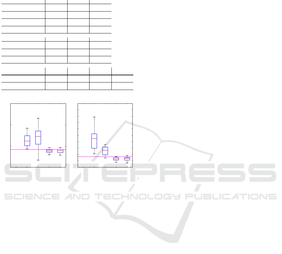
Table 3: Survey results for eight novice and one expert user

concerning the ease, usefulness, accuracy and rapidness of

the individual methods.

Question

Very easy [%] OK [%] Difﬁcult [%]

How easy was it to use the

DIRECT method?

55.6 22.2 22.2

How easy was it to use the

POINT support method?

88.9 11.1 0

How easy was it to use the

LINE support method?

100 0 0

How easy was it to use the

PLANE support method?

100 0 0

Question

Yes [%] Not sure [%] No [%]

Do you think the POINT

support method is useful?

44.4 44.4 11.1

Do you think the LINE

support method is useful?

77.8 22.2 0

Do you think the PLANE

support method is useful?

88.9 11.1 0

Question

Direct [%] Point support

[%]

Line support

[%]

Plane support

[%]

Which method do you prefer for

ACCURATE measurements?

0 0 44.4 55.6

Which method do you prefer for

FAST measurements?

11.1 22.2 44.4 22.2

direct_ref

direct

point

line

plane

Method

2.15

2.2

2.25

2.3

Distance [m]

Box plot of measured distances

direct_ref

direct

point

line

plane

Method

1.7

1.72

1.74

1.76

1.78

1.8

1.82

1.84

1.86

1.88

1.9

Area [m

]

Box plot of measured areas

Figure 8: Pilot study results: distances between the two ﬁrst

window corners (left) and areas of the window (right) (out-

liers removed before evaluation). The plots show the me-

dian of the distance and area measurements, the lower and

upper extremes, the 25

and the 75

percentile. The hori-

zontal lines are the reference distance and area.

ing a RANSAC scheme on multiple measurements),

and to further improve the GUI to more intuitively

and automatically guide users through the measure-

ment process.

We want to emphasize that, despite the basic al-

gorithmic concepts are known for years, practical ap-

plications are still largely missing due to the issues

arising in real measurement situations. As shown in

this work, it is therefore highly relevant to study these

concepts in practice to identify and overcome short-

comings of the underlying algorithms.

ACKNOWLEDGEMENTS

This work was funded by a grant from the Compe-

tence Centers for Excellent Technologies (COMET)

843272 with support from Hilti AG.

REFERENCES

Amann, M.-C., Bosch, T. M., Lescure, M., Myllylae, R. A.,

and Rioux, M. (2001). Laser ranging: a critical review

of usual techniques for distance measurement. Optical

Engineering, 40(1):10–19.

Braden, B. (1986). The Surveyor’s Area Formula. The Col-

lege Mathematics Journal, 17(4):326.

Coaker, L. H. (2009). Reﬂectorless Total Station Measure-

ments and their Accuracy, Precision and Reliability.

B.S. Thesis, University of Southern Queensland.

Criminisi, A., Reid, I., and Zisserman, A. (2000). Single

view metrology. International Journal of Computer

Vision, 40(2):123–148.

Ehrhart, M. and Lienhart, W. (2015). Image-Based Dy-

namic Deformation Monitoring of Civil Engineering

Structures from Long Ranges. Image Processing:

Machine Vision Applications VIII, 9405(1):94050J–

94050J–14.

Fathi, H. and Brilakis, I. (2013). A Videogrammetric As-

Built Data Collection Method for Digital Fabrication

of Sheet Metal Roof Panels. Advanced Engineering

Informatics, 27(4):466–476.

Fischler, M. A. and Bolles, R. C. (1981). Random Sample

Consensus: A Paradigm for Model Fitting with Ap-

plications to Image Analysis and Automated Cartog-

raphy. Commun. ACM, 24(6):381–395.

Hartley, R. and Zisserman, A. (2003). Multiple View Geom-

etry in Computer Vision. Cambridge University Press,

Cambridge, UK New York.

ISO 17123-3:2001 (2001). ISO 17123-3: Optics and opti-

cal instruments – Field procedures for testing geode-

tic and surveying instruments. Standard, International

Organization for Standardization, Geneva, CH.

Jadidi, H., Ravanshadnia, M., Hosseinalipour, M., and Rah-

mani, F. (2015). A Step-by-Step Construction Site

Photography Procedure to Enhance the Efﬁciency of

As-Built Data Visualization: A Case Study. Visual-

ization in Engineering, 3(1):1–12.

Juretzko, M. (2004). Reﬂektorlose Video-Tachymetrie ein

integrales Verfahren zur Erfassung geometrischer und

visueller Informationen. PhD thesis, Ruhr University

Bochum, Faculty of Civil Engineering.

Klasing, K., Althoff, D., Wollherr, D., and Buss, M. (2009).

Comparison of surface normal estimation methods for

range sensing applications. 2009 IEEE International

Conference on Robotics and Automation, pages 3206–

3211.

Leys, C., Ley, C., Klein, O., Bernard, P., and Licata, L.

(2013). Detecting outliers: Do not use standard devi-

ation around the mean, use absolute deviation around

the median. Journal of Experimental Social Psychol-

ogy, 49(4):764–766.

Martin, D. and Gatta, G. (2006). Calibration of total stations

instruments at the ESRF. Proceedings of XXIII FIG

Congress, pages 1–14.

Nichols, J. M. and Beavers, J. E. (2003). Development and

Calibration of an Earthquake Fatality Function. Earth-

quake Spectra, 19(3):605–633.

VISAPP 2017 - International Conference on Computer Vision Theory and Applications

Reda, A. and Bedada, B. (2012). Accuracy analysis and

Calibration of Total Station based on the Reﬂectorless

Distance Measurement. Master’s thesis, Royal Insti-

tute of Technology (KTH), Sweden.

Scherer, M. (2001). Advantages of the Integration of Im-

age Processing and Direct Coordinate Measurement

for Architectural Surveying - Development of the Sys-

tem TOTAL. FIG XXII International Congress.

Scherer, M. (2004). Intelligent Scanning with Robot-

Tacheometer and Image Processing: A Low Cost Al-

ternative to 3D Laser Scanning? FIG Working Week.

Scherer, M. and Lerma, J. L. (2009). From the Conven-

tional Total Station to the Prospective Image Assisted

Photogrammetric Scanning Total Station: Compre-

hensive Review. Journal of Surveying Engineering,

135(4):173–178.

Schneider, D. (2009). Calibration of a Riegl LMS-Z420i

based on a multi-station adjustment and a geomet-

ric model with additional parameters. The Interna-

tional Archives of the Photogrammetry, Remote Sens-

ing and Spatial Information Sciences 38 (Part 3/W8),

XXXVIII:177–182.

Schneider, P. and Eberly, D. (2003). Geometric Tools for

Computer Graphics. Boston Morgan Kaufmann Pub-

lishers, Amsterdam.

Schulz, T. (2007). Calibration of a Terrestrial Laser

Scanner for Engineering Geodesy. PhD thesis, ETH

Zurich, Switzerland.

Siu, M.-F., Lu, M., and AbouRizk, S. (2013). Combining

Photogrammetry and Robotic Total Stations to Obtain

Dimensional Measurements of Temporary Facilities

in Construction Field. Visualization in Engineering,

1(1):4.

Topcon Corporation (2011). Imaging Station IS Series, In-

struction Manual.

Uren, J. (2010). Surveying for Engineers. Palgrave Macmil-

lan, Basingstoke England New York.

Zeiske, K. (2004). Surveying made easy. https://www1.aps.

anl.gov/ﬁles/download/DET/Detector-Pool/

Beamline-Components/Lecia Optical Level/

Surveying en.pdf.

Measuring Human-made Corner Structures with a Robotic Total Station using Support Points, Lines and Planes