
A Three-dimensional Error-diffusion Algorithm for Importance
Sampling with Blue-noise Property
Ke Wang, Jiaojiao Zhao, Jie Feng and Bingfeng Zhou
Institute of Computer Science and Technology, Peking University, Beijing, China
Keywords:
Error-diffusion, Blue-noise, Importance Sampling, Volume Rendering.
Abstract:
We propose a novel discrete three-dimensional sampling algorithm based on the error-diffusion method, which
can generate sampling points with blue-noise property. To obtain sampling points with a high quality blue-
noise spectrum in 3D domain, we introduce an effective metric for the 3D blue-noise property based on 3D
Fourier transform. Then, a cost function used for the search of optimal parameters, including optimal diffusion
coefficients and threshold modulation strength values, is designed to guarantee the blue-noise property of
sampling points. Experiments show that our algorithm is able to generate sampling points with uniform
and random distribution, which possess 3D blue-noise property, and supports importance sampling in three
dimensional domain. Comparing with similar work, our algorithm can achieve sampling point distribution
that possesses better isotropic properties and has lower time cost in 3D discrete domain. Several applications
including volume rendering and tetrahedral meshing are also explored.
1 INTRODUCTION
Sampling is an important technique employed in
many computer graphics applications such as halfton-
ing, rendering, vectorization, physically-based sim-
ulation and geometry processing. Early research
include the Metropolis method (Metropolis et al.,
1953), Poisson disk sampling (Cook, 1986) and Cen-
troidal Voronoi Tessellation (CVT) (Du et al., 1999).
Blue-noise property refers to a sampling point dis-
tribution that is random, even and isotropic. It is char-
acterized by a symmetrical frequency spectrum that
lacks the power in low frequency. Originally blue-
noise property (Ulichney, 1987) is used to measure
the quality of a sampling algorithm in 2D domain.
More recently, blue-noise sampling is widely used for
stippling and remeshing in computer graphics (Yan
et al., 2015), which extends its application to higher
dimensions.
Among these high dimensional applications, vol-
ume rendering is a typical one where 3D sampling
plays an important role. The volume data generated
by modern 3D scanning technologies, such as CT and
MRI (Novelline and Fisher, 2004), is discrete and
located at regular grid points. The size of the acquired
data is often drastically large, and seriously affects
This work is partially supported by NSFC grants
#61370112, #61602012.
the efficiency of rendering and other processing of
the volume data. An optimized sampling to the
volume data can greatly reduce its size, while main-
taining the key features of the data. Similar works
include Monte Carlo volume rendering (Csebfalvi
and Szirmay-Kalos, 2003) and particle-based volume
rendering (Sakamoto et al., 2007). In these studies,
a point cloud of random samples is first generated
and then rendered to efficiently visualize large volume
data sets.
Poisson disk sampling (Dipp
´
e and Wold, 1985;
Cook, 1986) is a widely used method to generate
sampling points with the blue-noise property. How-
ever, the time complexity of the algorithm is high,
especially when the number of sampling points is
large. Recent studies, including SPH-based sam-
pling (Jiang et al., 2015) and kernel-based sampling
method (Zhong and Hua, 2016), can also be applied
in 3D sampling. Error-diffusion algorithm (Floyd and
Steinberg, 1976) is an important sampling method
working on discrete domain. It has high efficiency,
since it is independent of the number of sampling
points. Zhou and Fang made some improvements on
the original error-diffusion (Zhou and Fang, 2003),
so that high quality sampling points with blue-noise
distribution can be quickly generated.
Considering both the efficiency and the quality,
we propose a three-dimensional error-diffusion algo-
70
Wang K., Zhao J., Feng J. and Zhou B.
A Three-dimensional Error-diffusion Algorithm for Importance Sampling with Blue-noise Property.
DOI: 10.5220/0006097700700081
In Proceedings of the 12th International Joint Conference on Computer Vision, Imaging and Computer Graphics Theory and Applications (VISIGRAPP 2017), pages 70-81
ISBN: 978-989-758-224-0
Copyright
c
2017 by SCITEPRESS – Science and Technology Publications, Lda. All rights reserved
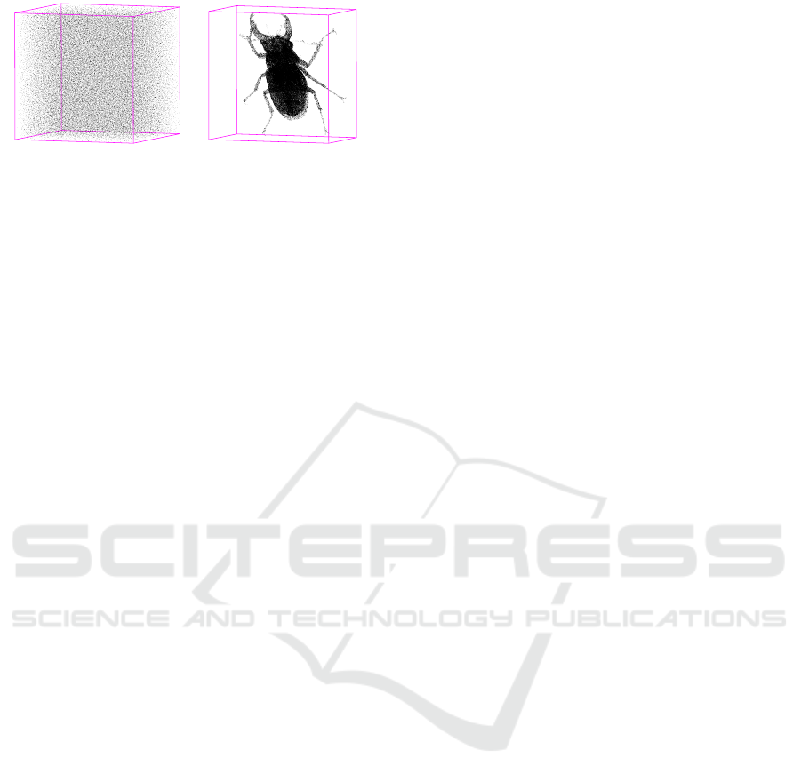
(a) Fixed-density (b) Variable-density
Figure 1: 3D error-diffusion sampling on discrete volume
data. (a) Uniform sampling on a 128
3
cube with a fixed
sampling density of g =
8
255
. (b) Importance sampling on a
set of volume data with variable sampling density.
rithm, which extends the original 2D error-diffusion
algorithm into 3D domain. Sampling points with 3D
blue-noise property can be generated by optimizing
the error-diffusion parameters. The algorithm is com-
putationally efficient and experimental results show
that sampling points with high quality 3D blue-noise
spectrum can be obtained (Fig.1). In particular, in this
paper we make the following contributions:
• We propose the framework of 3D error-diffusion,
including the scanning order, the quantization
threshold, the diffusion directions and diffusion
coefficients.
• In order to optimize the distribution of sampling
points, we introduce an effective metric of 3D
blue-noise property.
• During the search of optimal parameters, a cost
function is designed to obtain better blue-noise
property of sampling points. Experimental results
using these optimal parameters validate their ef-
fectiveness.
• We also demonstrate the applications of our
method in various areas, such as volume
rendering and tetrahedral meshing.
2 RELATED WORK
Poisson Disk Sampling. One of the original sam-
pling algorithm with blue-noise property is Poisson
disk sampling (Cook, 1986). A typical implemen-
tation of Poisson disk sampling is the dart throwing
method (Dipp
´
e and Wold, 1985; Cook, 1986), which
generates unbiased point distribution with minimum
distance constraints. Tile based methods (Cohen
et al., 2003; Ostromoukhov et al., 2004) improved the
efficiency by sacrificing bias-free condition, which
can not completely guarantee the blue-noise property
of the sampling output. Other methods have been
proposed to improve the performance, including hi-
erarchical dart throwing (White et al., 2007) and two
phase-algorithm (Ebeida et al., 2011).
Higher dimensional sampling is also important,
therefore Poisson disk sampling is extended to three,
four and even higher dimensions, utilizing parallel
multi-resolution uniform grid (Wei, 2008), spatial
subdivision (Gamito and Maddock, 2009) and flat
quadtree method (Ebeida et al., 2012). These methods
are able to generate sampling points with blue-noise
distribution for high dimension cases, but their perfor-
mance drops rapidly as the dimension increases.
Error-diffusion. The original error-diffusion is
an algorithm invented for generating halftone
images (Floyd and Steinberg, 1976). It is also
used in many other areas in computer graphics
as a sampling algorithm (Alliez et al., 2002;
Bourguignon et al., 2004; Kim et al., 2009).
Ulichney proposed serpentine error-diffusion with
threshold modulation for improving the output
quality (Ulichney, 1987). According to the analysis
of Knox and Eschbach (Knox and Eschbach, 1993),
threshold modulation is a kind of high frequency
perturbation to sampling points, which can reduce
grainy effect in the sampling output. Some other
research focused on ensuring the blue-noise property
of sampling points, including the variable-coefficient
error-diffusion (Ostromoukhov, 2001) and the
variable-threshold error-diffusion algorithm (Zhou
and Fang, 2003).
Unlike the error-diffusion which works directly
on a discrete domain, Poisson disk sampling (Cook,
1986) is originally designed in a continuous domain
and the algorithms are more complicated in higher
dimensions. Hence it is not suitable for certain
application areas that deal with 3D discrete domain.
Error-diffusion with variable coefficients and thresh-
olds (Zhou and Fang, 2003) can generate high quality
sampling point distribution that possess blue-noise
property. Moreover, the method can achieve linear
time complexity by using linear scanning order. For
these reasons, in this paper we propose a three-
dimensional sampling algorithm based on the stan-
dard 2D error-diffusion implementations.
3 THREE-DIMENSIONAL
ERROR-DIFFUSION
Our 3D error-diffusion is a sampling method for
discrete volume data, which can generate sampling
points with 3D blue-noise property. Discrete volume
data, composed of a set of voxels, is a very common
format for representing 3D physical signals in a dig-
A Three-dimensional Error-diffusion Algorithm for Importance Sampling with Blue-noise Property
71
Quantizationf(x, y, z) b(x, y, z)
Error filter
+
+
+
−
t(g)
e(x, y, z)
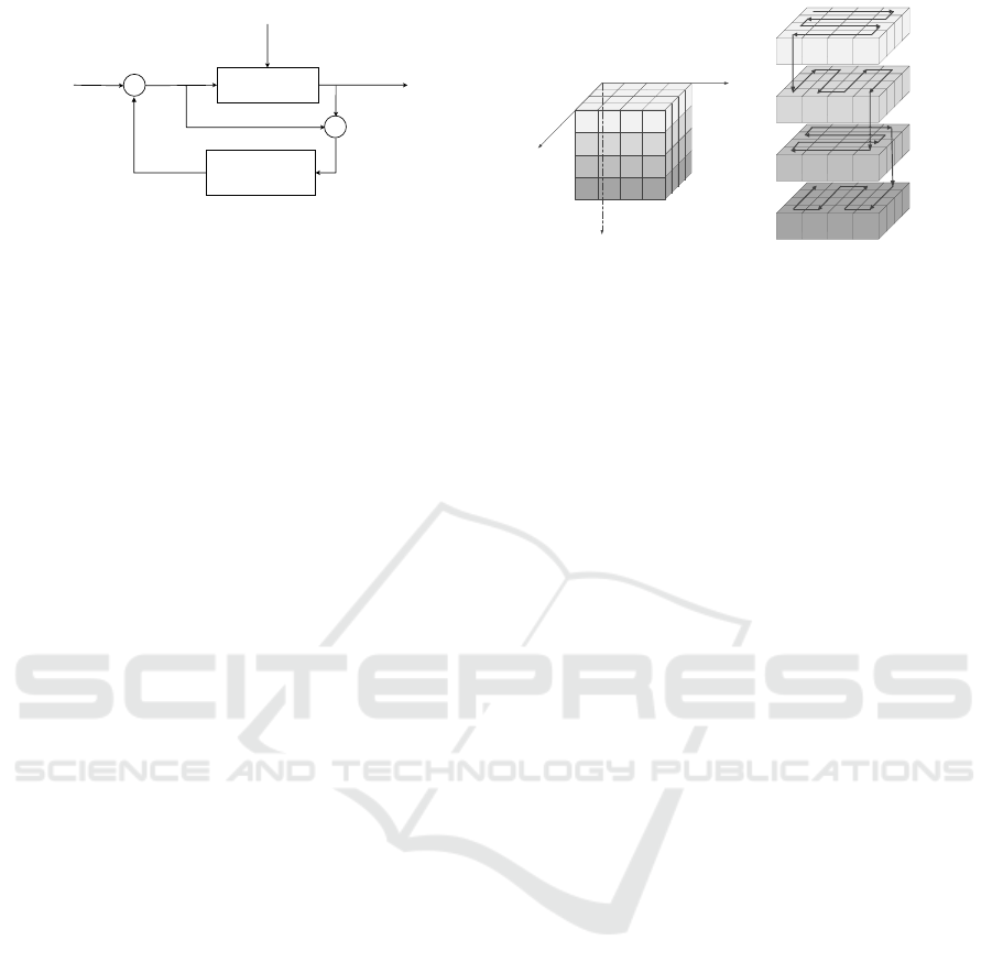
Figure 2: The framework of 3D error-diffusion. The input
sampling density is quantized by a modulated threshold.
The quantization error is distributed into multiple un-
process voxels through an error filter, and finally results in
a binary output.
ital way. The aim of our algorithm is to optimally
generate sampling points that preserve characteristics
of the original volume data for further processing,
e.g., volume rendering and tetrahedral meshing.
For this purpose, the intensity of the volume data
is first normalized and converted into a sampling
densitywhose time complexity is linear with respect
to the input data size. Hence, we assume that the input
volume data is available as a finite number of density
values g = f (x,y,z) located at regular grid points
(x,y,z). As described in Fig.2, the framework of 3D
error-diffusion is mainly composed of two steps:
• Quantization: Scanning the voxels according to a
specified scanning order, the quantization process
compares the input density value of each voxel
to a modulated quantization threshold t(g), and
return 0 if below, or 1 otherwise.
• Diffusion: The Quantization process produces an
error e(x,y,z) that is the difference between the
input and the output voxel density. Then the
error is distributed into neighboring un-processed
voxels through an error filter, which consists of a
set of diffusion coefficients.
Then the output b(x,y, z) forms a 3D binary volume
data, which includes black voxels whose density
is 1, representing the sampling points, and white
voxels otherwise, representing non-sampling points.
Hence, there are three main issues in the 3D error-
diffusion framework: (1) The scanning order; (2) The
quantization threshold; (3) The error filter, i.e., the
error-diffusion directions and coefficients.
Scanning Order. In the standard 2D error-diffusion,
serpentine scanning is a commonly used scanning
order (Ulichney, 1987; Ostromoukhov, 2001; Zhou
and Fang, 2003), which is able to remove the di-
rectional artifact caused by uni-directional scanning.
In 3D error-diffusion, the artifact should also be
avoided. For this purpose, we employ a similar
scheme in choosing the scanning order, which extends
the serpentine scanning to three-dimensional.
x
y
z
(a) A scanning cycle
Layer-1
Layer-3
Layer-2
Layer-4
(b) The scanning order
Figure 3: The rotated-serpentine scanning order. (a) A
scanning cycle includes four layers of volume data. (b)
Each layer adopts a different serpentine scanning direction.
Specifically, our algorithm scans voxels of the
input volume in a top-bottom sequence, i.e., layers
of the input voxels are processed from top to bottom
one by one (Fig.3). Within each layer, voxels are
scanned in a rotated serpentine order. To perform
this, every four adjacent layers from top to bottom
in the input volume are grouped as one scanning
cycle (Fig.3(a)), where the scanning direction of 2D
serpentine scanning are rotated respectively by 90
◦
for each layer (Fig.3(b)).
Quantization Threshold. The quantization threshold
is a key element in the error-diffusion algorithm. In
its original form, it is a fixed value at the middle
of the dynamic range of the input signal. In order
to improve the blue-noise property of the output, it
becomes variable by introducing a threshold modu-
lation (Ulichney, 1987). In 3D error-diffusion, we
choose a threshold modulation function that is similar
with the one in the variable-threshold error-diffusion
algorithm (Zhou and Fang, 2003):
t(g) = 0.5 + r ·m(g), (1)
where g = f (x,y,z) is the density level of an input
voxel, t(g) is the quantization threshold, m(g) ∈ [0, 1]
is a density-dependent modulation strength, and r ∈
[0.0,1.0] is a white-noise random number. Similar
with the work (Zhou and Fang, 2003), but specific
to 3D error-diffusion, here we use a different mod-
ulation strength obtained by the optimization method
described in next section.
Error-diffusion Directions and Coefficients. In 2D
domain, blue-noise property is characterized by a
round shaped Fourier power spectrum. The diffusion
of the errors along the diffusion directions contributes
to the round shaped spectrum. Similarly, in 3D
domain, blue-noise property can be characterized by
a spherical shaped 3D Fourier power spectrum. In
order to obtain such a spectrum, we need to choose
appropriate 3D diffusion directions and coefficients
GRAPP 2017 - International Conference on Computer Graphics Theory and Applications
72
V
y
z
V
z
x
Scanning
V
y
x
( , )
01
xy
d
( , )
11
xy
d
( , )
01
xz
d
( , )
11
xz
d
( , )
10
yz
d
( , )
01
yz
d
( , )
11
yz
d
Scanning
( , )
10
xz
d
( , )
10
xy
d
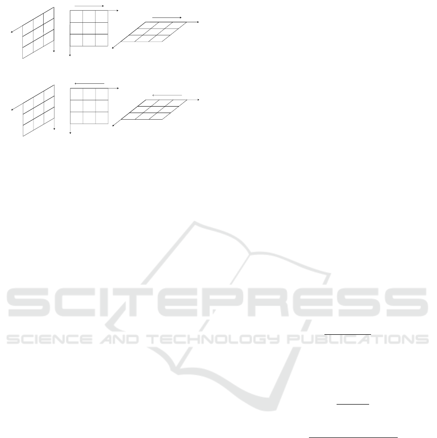
(a) The first diffusion direction of the layer-1
V
y
z
V
z
x
Scanning
V
y
x
( , )
01
xy
d
( , )
11
xy
d
( , )
01
xz
d
( , )
11
xz
d
( , )
10
yz
d
( , )
01
yz
d
( , )
11
yz
d
Scanning
( , )
10
xz
d
( , )
10
xy
d
(b) The second diffusion direction of the layer-1
Figure 4: The diffusion directions of the layer-1 in each
scan cycle.
by combining the three coordinate axes.
Specifically, for our 3D error-diffusion, there are
four sets of error filter configurations, corresponding
to the four rotated-serpentine scanning orders in a
scanning cycle. Taking the scanning order in layer-
1 as an example, we assume that current scanning
direction is along the increasing direction of the x
axis, and the scanning direction of y and z axis are
along increasing direction of the corresponding axis,
respectively. Then, the design of error filter given
in the standard 2D error-diffusion (Ostromoukhov,
2001; Zhou and Fang, 2003) is applied into three
coordinate planes, respectively. The corresponding
configuration of diffusion directions and coefficients
is shown in Fig.4. Considering the space relationship
of the three filters placed on the coordinate planes,
some of the coefficients are equal: d
(x,y)
01
= d
(y,z)
10
,
d
(x,y)
10
= d
(x,z)
10
, and d
(x,z)
01
= d
(y,z)
01
. Hence, there are
totally six independent coefficients for achieving an
output with blue-noise property. In our framework,
these coefficients are functions of the input density,
and can be determined by the optimization method
given in the next section.
For other layers of the scanning cycle, the cor-
responding diffusion directions can be obtained ac-
cordingly by aligning the same filters on different
scanning directions.
4 ERROR-DIFFUSION
PARAMETERS OPTIMIZATION
In the case of 2D error-diffusion, metrics are devel-
oped to evaluate the quality of the blue-noise property
of the output (Ostromoukhov, 2001; Zhou and Fang,
2003). In our 3D error-diffusion, similar metric is also
needed to obtain optimal parameters, including dif-
fusion coefficients and threshold modulation strength
values. In this section, we first define the metric of
3D blue-noise property, and then propose the method
of parameter optimization based on the metric.
4.1 Three-dimensional Blue-noise
The property of a sampling point set can be evalu-
ated by its Fourier power spectrum. To obtain the
Fourier power spectrum, we first perform 3D Fourier
transform on the sampling points, using a multi-
dimensional fast Fourier transform algorithm (Press
et al., 1992). Therefore, a 3D Fourier power spectrum
ˆ
P( f ) is calculated, where f is a 3D frequency vector.
Analogous to the definition of 2D blue-noise, 3D
blue-noise also refers to the noise whose energy is
absent in low frequency region, while the spectrum
is symmetrical in high-frequency region. The cor-
responding sampling points with blue-noise property
are scattered both randomly and evenly in the domain.
Based on these analysis, we propose a method for
measuring the blue-noise property of 3D sampling
point distributions.
In (Ulichney, 1987), the radially averaged power
spectrum and anisotropy are defined as the metrics
of 2D blue-noise property. Similarly, we define
the radially averaged power spectrum of 3D Fourier
power spectrum as
P( f
r
) =
∑
N( f
r
)
i=1
ˆ
P( f
i
)
N( f
r
)
, (2)
where N( f
r
) is the number of frequency samples on
the spherical shell of radius r. Also, the anisotropy
anis( f
r
) of 3D Fourier power spectrum is defined as
anis( f
r
) =
var
2
( f
r
)
P
2
( f
r
)
, (3)
var
2
( f
r
) =
∑
N( f
r
)
i=1
(
ˆ
P( f
i
) −P( f
r
))
2
N( f
r
) −1
. (4)
where var
2
( f
r
) is the variance of the power spectrum
ˆ
P( f ) on the spherical shell of radius r.
To obtain a better sampling point distribution, the
frequency spectrum should have a spherical symmet-
ric distribution and lack low frequency energy, and
this can be achieved by searching for optimal pa-
rameters. In the following sections, a corresponding
optimization target function is described on the basis
of our 3D blue-noise metrics.
4.2 Searching for Optimal Parameters
As the target of the optimization, the optimal parame-
ters should lead to a symmetrical frequency spectrum,
A Three-dimensional Error-diffusion Algorithm for Importance Sampling with Blue-noise Property
73
which should be as close as possible to 3D blue-
noise frequency spectrum. Derived from the 2D error-
diffusion algorithm, a target function for optimal
parameter searching is formulated as a weighted sum
of two parts:
T (g) = w ·L(g) + (1 −w) ·S(g). (5)
The first part is the low frequency ratio L(g), which
measures the similarity of the output spectrum with
the ideal 3D blue-noise frequency spectrum. The
second part S(g) is the similarity of the segmented
radially averaged power spectrums (SRAPSs) (Zhou
and Fang, 2003), which measures the symmetry of
the output frequency spectrum. w is a weight (0 ≤
w ≤ 1) determined according to the convergence of
parameter searching.
The Low Frequency Ratio. L(g) is calculated as
the ratio between the spectrum energy below the
principal frequency and the energy of the whole
spectrum.
For a 2D blue-noise distribution with dot density
g, the relationship between the principal frequency f
g
and the average dot distance λ
g
has the form of f
g
=
1/λ
g
= u ·
√
g, where u is a constant (Ulichney, 1987).
Similar analysis for 3D blue-noise point distributions,
which can be found in Appendix A, reveals that this
relationship takes a similar form in 3D domain, as
given in Eq.6:
f
g
=
(
3
√
g 0 ≤g ≤ 0.5,
3
p
1 −g 0.5 ≤ g ≤1.
(6)
Thus, the low frequency ratio L(g) for sampling
points with a density level of g, can be presented by
L(g) =
∑
f
g
f =0
ˆ
P( f )
∑
√
3/2
f =0
ˆ
P( f )
. (7)
Since L(g) is the ratio between the energy of low
frequencies and the total energy of all frequencies, it
is a value between 0 and 1. When L(g) is close to 0, it
indicates that the low frequency energy of the Fourier
power spectrum is close to zero. That is an important
indication of 3D blue-noise property.
The Symmetry of Frequency Spectrum. The sec-
ond part of the target function concerns the symmetry
of the Fourier power spectrum. Here, we consider the
symmetry of a 3D frequency spectrum in one of the
eight octants, and take it as another indication of 3D
blue-noise property.
We employ the concept of the segmented power
spectrum from 2D error-diffusion (Zhou and Fang,
2003) and give it a new definition in 3D domain. First,
the octant of the Fourier power spectrum domain is
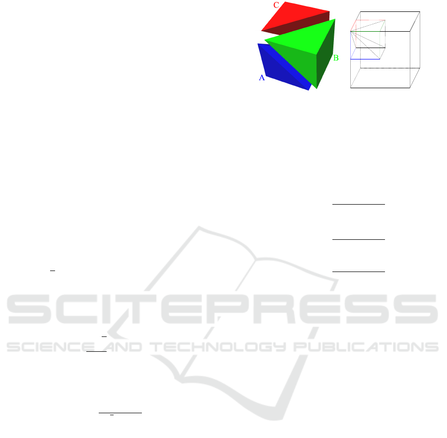
A
B
C
B
A
C
Figure 5: An octant of Fourier domain is symmetrically
divided into three equal pyramids for calculating the
segmented radially averaged power spectrums (SRAPSs).
divided into three equal segments which are defined
by the pyramids A, B and C as shown in Fig.5.
Then, for each segment, the SRAPSs are calculated
as following, respectively:
P
xy
( f
r
) =
∑
N
xy
( f
r
)
i=0
ˆ
P( f
i
)
N
xy
( f
r
)
, (8)
P
xz
( f
r
) =
∑
N
xz
( f
r
)
i=0
ˆ
P( f
i
)
N
xz
( f
r
)
, (9)
P
yz
( f
r
) =
∑
N
yz
( f
r
)
i=0
ˆ
P( f
i
)
N
yz
( f
r
)
. (10)
Here, P
xy
( f
r
),P
xz
( f
r
),P
yz
( f
r
) are three SRAPSs
corresponding to the pyramids A, B and C, and
N
xy
( f
r
),N
xz
( f
r
),N
yz
( f
r
) denote the number of
frequency samples for frequency f
r
in the three
pyramids, respectively.
We assume that correlation of these SRAPSs is an
indication of the symmetry of the whole spectrum.
Therefore, our similarity function S(g) of the three
SRAPSs is defined as
S(g) = 1 −C(P
xy
,P
xz
,P
yz
). (11)
Here, C is the correlation function (Gonzalez et al.,
2004) of the three curves P
xy
( f
r
),P
xz
( f
r
),P
yz
( f
r
). The
larger its value is, the more similar the curves are.
Parameter Optimization. With L(g) and S(g) de-
fined, the target function T (g) in Eq.5 can be cal-
culated. When the target function takes smaller
value, the frequency spectrum is closer to a 3D blue-
noise frequency spectrum. Therefore, the optimal
parameters can be obtained for a given density g by
minimizing T (g).
When searching for the optimal error-diffusion
parameters, we consider only the density input within
[0,0.5]. For any density g ∈ [0.5,1], the optimal
diffusion parameter for the density 1 − g can be
directly used. It is because at this density level, we
concern only the distribution of the ‘minority voxels’
of the sampling domain, whose distribution pattern is
the same as that at level 1 −g.
GRAPP 2017 - International Conference on Computer Graphics Theory and Applications
74
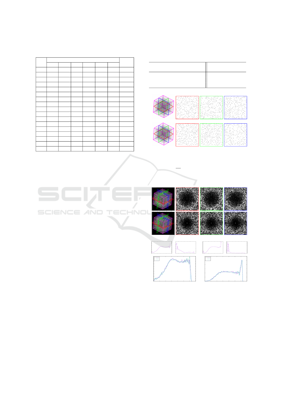
Table 1: The optimal error-diffusion parameters for key
density levels.
ˆg
k
Optimal Diffusion coefficients
m(g)
A
100
A
-110
A
010
A
0-11
A
-101
A
001
1 380 79 270 62 72 59 1.00
8 525 319 719 291 132 204 1.19
16 355 202 394 171 213 110 1.09
24 338 211 240 196 164 114 1.06
32 187 179 403 132 170 144 0.99
40 163 84 394 127 236 102 1.04
48 181 90 317 75 110 154 0.93
56 114 141 446 110 211 163 1.04
64 169 99 321 101 103 154 0.89
72 225 251 221 199 54 164 0.98
80 164 209 419 236 41 179 1.06
88 130 212 498 203 54 198 1.05
96 228 209 325 140 314 380 1.01
104 173 104 368 67 65 203 0.94
112 122 184 436 109 234 166 1.09
120 75 225 535 82 129 236 1.02
127 366 322 324 80 125 283 1.23
In order to reduce the computational complexity,
we only calculate optimal parameters for a group of
selected key density levels. For each key density
level, the optimal parameters are found by minimizing
T (g) with a simplex optimization algorithm (Press
et al., 1992), and a weight w = 0.02 is used in our
implementation.
After the optimization for each key density g
k
,
a diffusion coefficient set and a modulation strength
value set are obtained and listed in Table 1. Here,
ˆg
k
= g
k
·255 is the key density level and m(g) is the
modulation strength value. The diffusion coefficients
are defined by A
100
, A
-110
, A
010
, A
0-11
, A
-101
and A
001
:
d
(x,y)
10
= d
(x,z)
10
= A
100
(g)/M(g), d
(x,y)
-11
= A
-110
(g)/M(g),
d
(x,y)
01
= d
(y,z)
10
= A
010
(g)/M(g), d
(y,z)
-11
= A
0-11
(g)/M(g),
d
(x,z)
01
= d
(y,z)
01
= A
001
(g)/M(g), d
(x,z)
-11
= A
-101
(g)/M(g),
where M(g) = A
100
+ A
-110
+ A
010
+ A
0-11
+ A
-101
+
A
001
. It can be found that some values of modulation
strength m(g) is slightly larger then 1.0. This is
acceptable because it simply amplifies the energy of
the added white noise. According to our experi-
ments, that can help to achieve better symmetry of
the Fourier power spectrum, and is not harmful to the
obtained sampling result (Knox and Eschbach, 1993;
Zhou and Fang, 2003).
For other density levels, the optimal parameters
can be quickly calculated by a linear interpolation
between their two adjacent key density levels.
Table 2: The average sampling efficiency of our method and
3D Poisson disk sampling methods (The volume data size
in our method is 128
3
).
Method
Number of samples
per second (3D)
(Gamito and Maddock, 2009) 10
3
∼ 10
4
(Ebeida et al., 2012) 7.5 ×10
4
Our method 10
6
∼ 10
7
Gamito Method
N = 16, 431
Our Method
N = 16, 471
Figure 6: The sampling results using our method and
3D Poisson disk sampling method (Gamito and Maddock,
2009). The volume data is a 64
3
cube with a fixed sampling
density of g =
16
255
in our method. N is the number of
sampling results. Locations of the 2D slices are indicated
by colors.
Gamito MethodOur Method
(a) Spectrum slices
0
50
100
150
200
250
300
0 10 20 30 40 50 60 70
0
0.5
1
1.5
2
2.5
3
3.5
0 10 20 30 40 50 60 70
0
20
40
60
80
100
120
140
160
180
200
0 10 20 30 40 50 60 70
XY
XZ
YZ
Gamito method
0
20
40
60
80
100
120
140
160
180
200
0 10 20 30 40 50 60 70
0
2
4
6
8
10
12
14
16
18
0 10 20 30 40 50 60 70
0
50
100
150
200
250
300
0 10 20 30 40 50 60 70
XY
XZ
YZ
Our method
(b) Spectrum statistics
Figure 7: Comparison of our method with 3D Poisson disk
sampling method (Gamito and Maddock, 2009) in terms of
Fourier power spectrum slices and statistics. (a) 3D Fourier
power spectrum slices of the sampling results (Fig.6). (b)
Top: radially averaged power spectrum and anisotropy.
Bottom: SRAPSs. The location of the 2D slices is indicated
by colors.
A Three-dimensional Error-diffusion Algorithm for Importance Sampling with Blue-noise Property
75
5 EXPERIMENTAL RESULTS
With the optimized parameters, our 3D error-
diffusion algorithm is able to generate sampling
points with blue-noise distribution. We implement
our sampling algorithm on a common PC with an
Intel i7 3.4GHz CPU. In this section, experimental
results of our algorithm are shown and analyzed.
5.1 Comparison with Poisson Disk
Sampling
We compare our 3D error-diffusion sampling method
with the Poisson disk sampling methods (Gamito and
Maddock, 2009; Ebeida et al., 2012). In Table 2,
we show the sampling efficiency of the two kind of
methods.
In fact, the time complexity of our method is
linear in the size of the input volume data, which is
independent of the input data set. Therefore, the time
complexity of our method is O(N
0
), where N
0
= L
3
is the size of the volume data. However, the time
complexity of the Poisson disk sampling method is
correlated positively with the number of sampling
points, and inversely with the disk radius. The time
complexity of Poisson disk sampling is O(NlogN) in
spatial subdivision (Gamito and Maddock, 2009) and
empirical Θ(N) in the flat quadtree method (Ebeida
et al., 2012). Therefore, when the number of sampling
points grows, the time cost of our method remains
constant, while that of 3D Poisson disk sampling
increases significantly.
The number of sampling points obtained by 3D
error-diffusion is determined by the average density.
For a volume data with fixed density level g and size
of L
3
, the expected number of sampling points N
satisfies
N = g ·L
3
. (12)
Given the same number of sampling points, both
kind of methods produce comparable sampling results
(Fig.6). The Fourier power spectrums and their 2D
slices demonstrate that the sampling points generated
by both methods are uniformly and randomly dis-
tributed (Fig.7(b)), and their frequency spectrums are
symmetrical and lack of low frequency component
(Fig.7(a)). However, when inspecting the spectrums
with the metrics defined in Section 4, we can find
that the sampling results by our method achieve better
blue-noise property. The SRAPS curves given in
Fig.7(b) indicate that our results have better symme-
tries than the 3D Poisson disk sampling method.
5.2 Volume Data with Fixed Sampling
Density
Fixed Params
Optimal Params
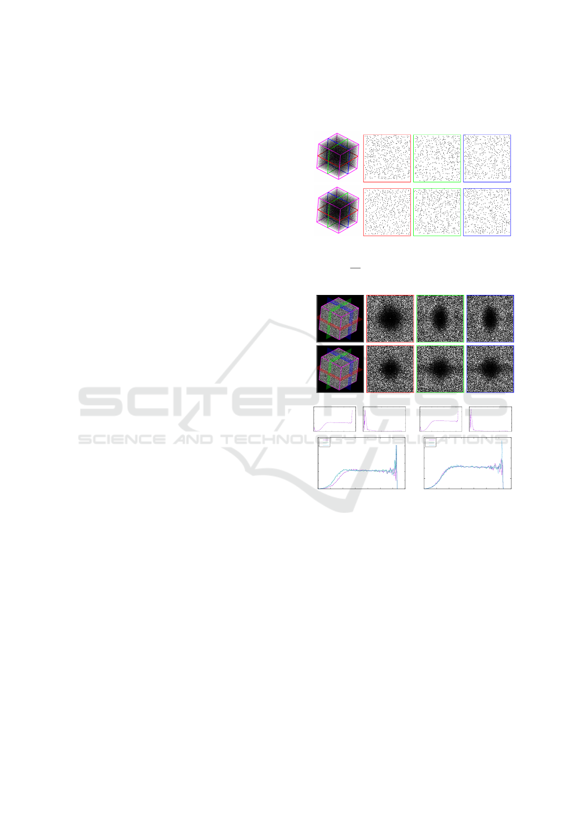
Figure 8: The sampling results using optimal parameters
and fixed parameters. The input volume data has a fixed
density g =
8
255
and the size of 128
3
. Locations of the 2D
slices are indicated by colors.
Fixed Params
Optimal Params
(a) Spectrum slices
0
50
100
150
200
250
300
0 20 40 60 80 100 120 140
0
5
10
15
20
25
30
0 20 40 60 80 100 120 140
0
50
100
150
200
250
300
0 20 40 60 80 100 120 140
XY
XZ
YZ
Fixed parameters
0
50
100
150
200
250
0 20 40 60 80 100 120 140
0
5
10
15
20
25
30
0 20 40 60 80 100 120 140
0
50
100
150
200
250
0 20 40 60 80 100 120 140
XY
XZ
YZ
Optimal parameters
(b) Spectrum statistics
Figure 9: Comparison of optimal parameters with fixed
parameters in terms of Fourier power spectrum slices and
statistics. (a) 3D Fourier power spectrum slices of the
sampling results (Fig.8). (b) Top: radially averaged power
spectrum and anisotropy. Bottom: SRAPSs. The location
of the 2D slices is indicated by colors.
To validate the effectiveness of our algorithm, we
compare the 3D sampling results using the optimal
variable parameters with that using the un-optimized
fixed parameters. In Fig.8 (top), fixed parameters
A
100
= 4, A
-110
= 2, A
010
= 4, A
0-11
= 2, A
-101
= 2,
A
001
= 2, and m(g) = 1.00 is used for sampling.
In this configuration, larger coefficients are given
to the closer diffusion positions to the voxel being
processed. In contrast, optimal parameters from
Table 1 are used in Fig.8 (bottom). The spectrum
statistical curves show that the optimal parameters
play an important role in improving the symmetry of
GRAPP 2017 - International Conference on Computer Graphics Theory and Applications
76
(a)
(b)
Figure 10: Slices of 3D error-diffusion sampling to a 64 ×
64×256 variable-density volume data. The density changes
from 1 to 0 along the z axis. (a) XZ-Slice. (b) YZ-Slice.
the Fourier power spectrum. When considering the
correlation of the SRAPSs (Fig.9 (b)), we can see
that the optimal parameters lead to larger correlation
value than the fixed parameters. Consequently, the
spectrum using optimal parameters is more symmet-
ric (Fig.9 (a)), and thus has better 3D blue-noise
properties.
From the sampling point distribution shown in
Fig.8, it can be found that there are less granular
points clustering in the results using the optimal
parameters than using the un-optimized ones. That
is also a result of our optimization process which
reduces the lower frequency component in Fourier
power spectrums.
5.3 Volume Data with Variable
Sampling Density
As illustrated in Fig.10, we apply 3D error-diffusion
sampling to a set of volume data whose density
gradually changes along one of the coordinate axes.
From the 2D slices of the sampling result, we can
see that the sampling points have uniform and random
distribution.
Using 3D error-diffusion algorithm, we also per-
form importance sampling to several sets of complex
3D volume data according to their local features.
First, the attribute information of each voxel in the
volume data is converted into normalized sampling
density level. The resulting sampling density function
in the 3D volume space is taken as the input of our
algorithm. Then, each voxel in the volume data
uses different optimal parameters for quantization and
error-diffusion, according to its corresponding sam-
pling density. By this way, an importance sampling
result, controlled by the sampling density function,
can be obtained.
As shown in the experimental results in Fig.11,
the sampling points are distributed uniformly in the
3D volume and maintain the structure features of
the volume data. It can be seen that, the regions
with salient features contain more sampling points
and the smooth regions with less features have less
sampling. With this effect, our method is able to
reduce the number of voxels in the volume data while
maintaining the key features.
From the experimental results, a sampling
point distribution satisfying 3D blue-noise property
can be obtained. In low frequency region of the
Fourier power spectrum, our method achieves better
blue-noise property than 3D Poisson disk sampling
method (Gamito and Maddock, 2009). In the high
frequency region, our method can also guarantee the
isotropic characteristics. Furthermore, the time cost
of this sampling method is reduced compared with
3D Poisson disk sampling methods.
6 APPLICATIONS
The proposed 3D error-diffusion sampling method
can be used for importance sampling, under the
control of a sampling density function. Because of
its high quality and high efficiency, this method may
have many potential applications, such as volume
rendering and tetrahedral meshing. In this section, we
demonstrate the implementations and experimental
results of our method in these application areas.
6.1 Volume Rendering
Since our 3D error-diffusion sampling method is able
to produce blue-noise sampling point distribution, it
can be used to improve the rendering quality for
many volume rendering methods, e.g., the particle-
based volume rendering (PBVR) method (Sakamoto
et al., 2007). PBVR takes tiny particles as render
primitives. The particles are generated from a given
3D scalar field based on a user-specified transfer func-
tion. Then, the final rendering results is calculated by
projecting these particles onto the image plane.
In fact, the particles are essentially a group of
random sampling points on 3D space according to
the scalar field. In the original work of PBVR,
they are generated in two ways: the hit-and-miss
method (Sakamoto et al., 2007) or the Metropolis
method (Metropolis et al., 1953). The former method
performs sampling to discrete volume data. However,
it can only produce white-noise sampling results,
which do not possess the good properties of blue-
noise distribution. Comparing with this method, us-
ing our 3D error-diffusion sampling may significantly
improve the distribution of the particles, and hence
better rendering results can be obtained as shown in
Fig.12(b). The second method, i.e., the Metropolis
method works in continuous domain and can produce
particles with better distribution. But similar to the
Poisson Disk sampling method, its computational
cost is relatively high. In contrast, our sampling
A Three-dimensional Error-diffusion Algorithm for Importance Sampling with Blue-noise Property
77
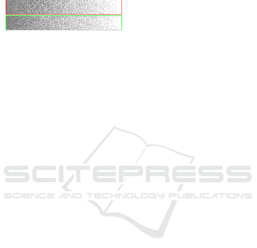
(a) Sampling Result (b) XY-Slice (c) XZ-Slice (d) YZ-Slice
Stag beetle
Present
Christmas tree
Figure 11: The 3D error-diffusion importance sampling results of variable-density volume data. The first column demonstrates
the sampling points from three different volume datasets, and the corresponding volume slices are shown in the right columns.
The volume datasets, Christmas Present (Heinzl, 2006), Stag Beetle (Gr
¨
oller et al., 2005) and Christmas Tree (Kanitsar, 2002),
courtesy of the Institut for computergraphik und Algorithmen, Technische Universit
¨
at Wien.
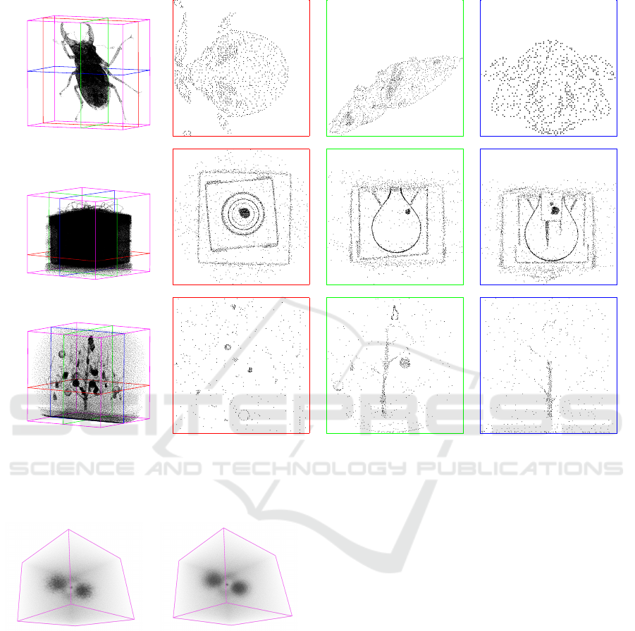
(a) Hit-and-miss method (b) Our method
Figure 12: Particle-based volume rendering results, with
particles generated by (a) Hit-and-miss method (Sakamoto
et al., 2007) and (b) our 3D error-diffusion sampling
method.
algorithm can guarantee the blue-noise property of the
particle distribution while the computing efficiency is
much higher.
In this way, our method can be applied to the areas
of volume rendering, in which a random sampling
point set on the volume with good distribution proper-
ties are necessary. Since our algorithm can effectively
maintain the blue-noise property, the volume render-
ing methods utilizing our method can achieve better
rendering results.
6.2 Volume Tetrahedral Meshing
In 2D image processing, vectorized image is a kind
of compact representation, and becomes an effective
alternative for traditional raster image. 2D image
vectorization method generates triangular meshes on
the image plane, based on a set of sampling points.
Similarly, vectorized represention for volume data is
also useful in many areas (Guo et al., 2016), and
tetrahedral meshing is a widely used 3D vectorization
method. First, a set of sampling points is generated
by sampling to the volume data. Then, tetrahedral
meshes are built from the sampling points. Obvi-
ously, the distribution property of the sampling points
directly affects the quality of the meshes.
Therefore, we also implement a volume tetrahe-
dral meshing method on the basis of our 3D error-
GRAPP 2017 - International Conference on Computer Graphics Theory and Applications
78
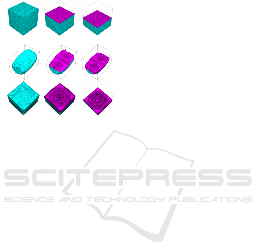
(a) Fixed-density volume data
(b) Variable-density volume data
Figure 13: Volume tetrahedral meshing based on our 3D
error-diffusion sampling points.
diffusion sampling method. The tetrahedral meshing
is performed based on the sampling points generated
by our method, and completed using the tools of
TetGen (Si, 2015). Fig.13 shows the experimental
results. First, a uniform tetrahedral mesh is built on
the sampling result of a fixed-density volume data
(Fig.13(a)). Then, two more complex tetrahedral
meshes are constructed based on the importance sam-
pling to the variable-density volume data (Fig.13(b)).
From the sliced views of the tetrahedral meshes, we
can see that the internal sampling points of the vol-
ume data are evenly distributed, hence the resulting
meshes have a regular tetrahedral structure.
On the vertices of each tetrahedron, the attribute
information of their corresponding original voxel,
such as color or density, can be directly stored. In the
internal of the tetrahedron, the attribute information
of each voxel can be calculated by a fast interpolation
according to the information stored on the four ver-
tices of the tetrahedron. This therefore forms a vector
expression of the original volume data. It can greatly
reduce the storage of volume data, and hence improve
the speed of volume transmission and rendering.
7 CONCLUSION
In this paper, a three-dimensional error-diffusion al-
gorithm is described, which is an extension of the
standard 2D error-diffusion. This algorithm can be
used for sampling over volume data where a 3D
discrete density function is defined at the voxels.
Similar with the tone-dependent 2D error-diffusion,
our algorithm is density-dependent, i.e., the diffusion
parameters are decided according to the density level
of the voxel being processed. By defining the metric
of 3D blue-noise property of sampling point distri-
butions, a set of optimal parameters for 3D error-
diffusion is obtained through an optimization process.
The parameter set includes diffusion coefficients and
threshold modulation strength values. Using the
optimized parameters, our 3D error-diffusion can
generate sampling points whose distribution possess
blue-noise property. The generated sampling points
shown in the bottom of Fig.8 possess a stochastic,
evenness and isotropic distribution, which can be
verified by Fig.9 (b). In this figure, the evenness and
low level of radial anisotropy means there is no out-
lied higher spectrum in frequency domain, which is
an indication of the property. The high correlation
and lack of low frequency within SRAPSs is also
an important indication of blue-noise property of the
point distribution.
To explore the applications of our algorithm, ex-
periments are also performed in the area of discrete
volume data processing, including volume rendering,
volume tetrahedral meshing. The results demonstrate
that our algorithm can generate high quality sampling
points with higher efficiency, and that can result in
better rendering and tetrahedral meshing for volume
data.
Limitation and Future Work. In our method, alias-
ing may occur at the beginning of the scanning
of our algorithm. That is because the cumulative
quantization error of the voxels is less than the dif-
fusion threshold at the beginning of sampling. This
transition effect should be further reduced in the
future work.
Exploring volume rendering based on the sam-
pling points will be another interesting future work.
Sampling points with 3D blue-noise distribution, as
well as corresponding tetrahedral meshes, can be
easily obtained by our method. The attributes of
the voxels inside a tetrahedron can be rapidly recon-
structed by interpolation method, such as mean value
coordinates (Ju et al., 2005). We will explore a fast
volume rendering method based on such tetrahedral
meshes, using new transfer functions, ray casting
integral methods, and hardware acceleration. Further
more, the tetrahedral meshes can be used to store and
reconstruct the original volume data, and is useful in
volume data compression.
A Three-dimensional Error-diffusion Algorithm for Importance Sampling with Blue-noise Property
79

REFERENCES
Alliez, P., Meyer, M., and Desbrun, M. (2002). Interactive
geometry remeshing. ACM Transactions on Graphics,
21(3):347–354.
Bourguignon, D., Chaine, R., Cani, M.-P., and Drettakis,
G. (2004). Relief: A modeling by drawing
tool. In Proceedings of the First Eurographics
Conference on Sketch-Based Interfaces and Modeling,
SBM’04, pages 151–160, Aire-la-Ville, Switzerland,
Switzerland. Eurographics Association.
Cohen, M. F., Shade, J., Hiller, S., and Deussen, O. (2003).
Wang tiles for image and texture generation. Acm
Transactions on Graphics, 22(3):287–294.
Cook, R. L. (1986). Stochastic sampling in computer
graphics. Acm Transactions on Graphics, 5(1):51–72.
Csebfalvi, B. and Szirmay-Kalos, L. (2003). Monte carlo
volume rendering. In Proc. IEEE Visualization 2003,
pages 449–456.
Dipp
´
e, M. A. Z. and Wold, E. H. (1985). Antialiasing
through stochastic sampling. SIGGRAPH Computer
Graphics, 19(3):69–78.
Du, Q., Faber, V., and Gunzburger, M. (1999). Centroidal
voronoi tessellations: Applications and algorithms.
SIAM Review, 41:637–676.
Ebeida, M. S., Davidson, A. A., Patney, A., Knupp, P. M.,
Mitchell, S. A., and Owens, J. D. (2011). Efficient
maximal poisson-disk sampling. Acm Transactions on
Graphics, 30(4):76–79.
Ebeida, M. S., Mitchell, S. A., Patney, A., Davidson, A. A.,
and Owens, J. D. (2012). A simple algorithm for
maximal poisson-disk sampling in high dimensions.
Computer Graphics Forum, 31(2):785–794.
Floyd, R. W. and Steinberg, L. (1976). An Adaptive
Algorithm for Spatial Greyscale. Proceedings of the
Society for Information Display, 17(2):75–77.
Gamito, M. N. and Maddock, S. C. (2009). Accurate
multidimensional poisson-disk sampling. ACM
Transactions on Graphics, 29(1):8:1–8:19.
Gonzalez, R. C., Woods, R. E., and Eddins, S. L. (2004).
Digital image processing using matlab. Ann.rev.fluid
Mech, 21(84):197–199.
Gr
¨
oller, M. E., Glaeser, G., and Kastner, J. (2005). Stag
beetle dataset. https://www.cg.tuwien.ac.at/research
/publications/2005/dataset-stagbeetle/.
Guo, J., Yan, D. M., Chen, L., Zhang, X., Deussen, O., and
Wonka, P. (2016). Tetrahedral meshing via maximal
poisson-disk sampling. Computer Aided Geometric
Design, 43:186–199.
Heinzl, C. (2006). Christmas present dataset. https://www.
cg.tuwien.ac.at/research/publications/2006/dataset-
present/.
Jiang, M., Zhou, Y., Wang, R., Southern, R., and Zhang,
J. J. (2015). Blue noise sampling using an sph-based
method. ACM Transactions on Graphics (TOG),
34(6):211.
Ju, T., Schaefer, S., and Warren, J. (2005). Mean value
coordinates for closed triangular meshes. ACM
Transactions on Graphics, 24(3):561–566.
Kanitsar, A. (2002). Christmas tree dataset. https://www.cg.
tuwien.ac.at/research/publications/2002/dataset-
christmastree/.
Kim, S. Y., Maciejewski, R., Isenberg, T., Andrews, W. M.,
Chen, W., Sousa, M. C., and Ebert, D. S. (2009).
Stippling by example. In Proc. the 7th International
Symposium on Non-Photorealistic Animation and
Rendering, NPAR ’09, pages 41–50.
Knox, K. T. and Eschbach, R. (1993). Threshold
modulation in error diffusion. Journal of Electronic
Imaging, 2(3):185–192.
Metropolis, N., Rosenbluth, A. W., Rosenbluth, M. N.,
Teller, A. H., and Teller, E. (1953). Equation of state
calculations by fast computing machines. Journal of
Chemical Physics, 21(6):1087–1092.
Novelline and Fisher, M. (2004). Squire’s fundamentals of
radiology, 6th ed.
Ostromoukhov, V. (2001). A simple and efficient error-
diffusion algorithm. In Proc. the 28th Annual
Conference on Computer Graphics and Interactive
Techniques, SIGGRAPH ’01, pages 567–572, New
York, NY, USA. ACM.
Ostromoukhov, V., Donohue, C., and Jodoin, P.-M. (2004).
Fast hierarchical importance sampling with blue
noise properties. ACM Transactions on Graphics,
23(3):488–495.
Press, W. H., Teukolsky, S. A., Vetterling, W. T., and
Flannery, B. P. (1992). Numerical Recipes in C (2nd
Ed.): The Art of Scientific Computing. Cambridge
University Press, New York, NY, USA.
Sakamoto, N., Nonaka, J., Koyamada, K., and Tanaka, S.
(2007). Particle-based volume rendering. In Proc.
Int’l Asia-Pacific Symposium on Visualization 2007,
APVIS ’07, pages 129–132.
Si, H. (2015). Tetgen, a delaunay-based quality
tetrahedral mesh generator. ACM Trans. Math. Softw.,
41(2):11:1–11:36.
Ulichney, R. (1987). Digital Halftoning. MIT Press,
Cambridge, MA.
Wei, L.-Y. (2008). Parallel poisson disk sampling. ACM
Transactions on Graphics, 27(3):20:1–20:9.
White, K. B., Cline, D., and Egbert, P. K. (2007). Poisson
disk point sets by hierarchical dart throwing. In Proc.
IEEE Symposium on Interactive Ray Tracing, pages
129–132.
Yan, D.-M., Guo, J.-W., Wang, B., Zhang, X.-P., and
Wonka, P. (2015). A survey of blue-noise sampling
and its applications. Journal of Computer Science and
Technology, 30(3):439–452.
Zhong, Z. and Hua, J. (2016). Kernel-based adaptive
sampling for image reconstruction and meshing.
Computer Aided Geometric Design, 43:68–81.
Zhou, B. and Fang, X. (2003). Improving mid-
tone quality of variable-coefficient error diffusion
using threshold modulation. ACM Transactions on
Graphics, 22(3):437–444.
GRAPP 2017 - International Conference on Computer Graphics Theory and Applications
80

APPENDIX
Derivation of the Principal Frequency
When density g of input volume data satisfies 0 ≤
g ≤ 0.5, average distance between sampling points
is called the principal wavelength (Ulichney, 1987).
If the principal wavelength is λ
g
, average volume
occupied by each sampling point is λ
3
g
. Therefore,
the number N of sampling points can be expressed by
following Eq.13:
N =
L
3
λ
3
g
(13)
where L is the size of the volume data. The number
N of sampling points can be obtained by Eq.12.
Therefore, the principal wavelength is derived as
following by equal of Eq.12 and Eq.13:
λ
g
=
1
3
√
g
(14)
where the density g satisfies 0 ≤g ≤0.5. Because the
principal frequency is the reciprocal of the principal
wavelength (Ulichney, 1987), the principal frequency
f
g
is described as follow:
f
g
=
3
√
g. (15)
Also, principal frequency f
g
can be obtained easily
when density g ∈ [0.5,1]. Therefore, the principal
frequency f
g
is described as Eq.6.
A Three-dimensional Error-diffusion Algorithm for Importance Sampling with Blue-noise Property
81
