
Nonlocal Regularizing Constraints in Variational Optical Flow
Joan Duran and Antoni Buades
Department of Mathematics and Computer Science, University of Balearic Islands, Cra. de Valldemossa km. 7.5,
07122 Palma, Illes Balears, Spain
Keywords:
Optical Flow, Motion Estimation, Variational Methods, Multiscale, Nonlocal Energy Terms, Total Variation.
Abstract:
Optical flow methods try to estimate a dense correspondence field describing the motion of the objects in an
image sequence. We introduce novel nonlocal regularizing constraints for variational optical flow computation.
While the use of similarity weights has been restricted to the regularization term so far, the proposed data
terms permit to implicitly use the image geometry in order to regularize the flow and better locate motion
discontinuities. The experimental results illustrate the superiority of the new constraints with respect to the
classical brightness constancy assumption as well as to nonlocal regularization strategies.
1 INTRODUCTION
Since the seminal works of Horn and Schunck (Horn
and Schunck, 1981) and Lucas and Kanade (Lucas
and Kanade, 1981), optical flow estimation has be-
come one of the most intensive research areas in com-
puter vision. The main objective of optical flow meth-
ods is to compute a dense correspondence field be-
tween an arbitrary pair of images in order to capture
the apparent dynamical behaviour of the objects in the
scene. This is a key step in several applications like
image registration, object tracking, robot navigation,
stereo reconstruction, or motion based segmentation.
Generally speaking, optical flow methods can be
classified into two large families. On the one hand,
local techniques establish point correspondences by
minimizing a distance measure matching small win-
dows (Lowe, 2004; Yoon and Kweon, 2006). These
methods commonly provide a sparse flow field due
to the lack of discrimination at certain points. On
the other hand, global or variational methods provide
a dense solution through the minimization of an en-
ergy in which the regularization term interconnects all
the pixels of the image, thus filling-in the flow wher-
ever no sufficient information is available (Brox et al.,
2004; Zach et al., 2007; Zimmer et al., 2009).
Variational optical flow methods require a con-
straint imposing the preservation of certain image fea-
tures over the trajectories. In this regard, the classical
hypothesis is the brightness constancy assumption,
which was already considered in the Horn-Schunck
and Lucas-Kanade models. However, this constraint
is very limiting because is not invariant to illumina-
tion changes. Robustness can be recovered by using
photometric invariant constraints, such as the gradi-
ent constancy assumption (Brox et al., 2004), higher-
order derivatives (Papenberg et al., 2006), patch-
based measures (Vogel et al., 2013), or alternative
color spaces (Zimmer et al., 2009; Mileva et al.,
2007). Several works (Alvarez et al., 2002; Kennedy
and Taylor, 2015) have also handled the characteri-
zation of occlusions, which is one of the major chal-
lenges in realistic scenarios.
Traditionally, variational techniques include a lin-
earization of the warped image in the data term in
order to minimize the energy. This linearization is
only valid for small displacements and, as a conse-
quence, the optimization is embedded in a coarse-
to-fine warping scheme (Black and Anandan, 1996;
M
´
emin and P
´
erez, 1998) to better capture large mo-
tions. On the contrary, the linearization is post-
poned to the numerical scheme in several works
(Nagel and Enkelmann, 1986; Brox et al., 2004;
Brox and Malik, 2011), illustrating significative per-
formance gain. Other approaches completely depart
from coarse-to-fine strategies. For instance, Stein-
br
¨
ucker et al. (Steinbr
¨
ucker et al., 2009) decouple the
data and the regularization terms by a quadratic relax-
ation and the optimization problem is directly solved
at the finest scale by alternating two global minimiza-
tions while decreasing the decoupling parameter.
Computing the displacement field is in general an
ill-posed problem and, thus, a priori knowledge on
the sought solution is required. This prior usually
Duran J. and Buades A.
Nonlocal Regularizing Constraints in Variational Optical Flow.
DOI: 10.5220/0006098501510161
In Proceedings of the 12th International Joint Conference on Computer Vision, Imaging and Computer Graphics Theory and Applications (VISIGRAPP 2017), pages 151-161
ISBN: 978-989-758-227-1
Copyright
c
2017 by SCITEPRESS – Science and Technology Publications, Lda. All rights reserved
151

takes the form of spatial smoothness which promotes
smoothing in regions of coherent motion while per-
mitting flow discontinuities. Nonlocal strategies have
also been proposed as regularization terms (Werl-
berger et al., 2010; Ranftl et al., 2014).
While the use of nonlocal similarity has been re-
stricted to the regularization term, we propose two
new fidelity terms for optical flow estimation that
make use of such a similarity configuration. The pro-
posed terms permit to implicitly use the image geom-
etry in order to regularize the flow and better locate
motion discontinuities. The first term regularizes the
flow by extending the classical brightness constancy
assumption to similar pixels. That is, the flow for
a certain pixel should be able to correctly match the
color of its most similar pixels. The second term aims
at replacing the classical assumption and no longer
matches points along the trajectory. It uses a weight
family across the two images in order to transfer patch
similarity to the flow. This might be seen as an alter-
native for combining classical optical flow and block
matching techniques.
The rest of the paper is organized as follows. In
Section 2, we review the state of the art in variational
optical flow computation. We derive the two novel
nonlocal regularizing constraints in Section 3. Sec-
tion 4 details the optimization strategy used for com-
puting the flow field. In Section 5, we display some
experimental results and we finish with some conclu-
sions in Section 6.
2 STATE OF THE ART
Let I : Ω ×[0, T] → R be an image sequence, where
Ω is a rectangular domain in R
2
and I(x,t) denotes
the intensity value at pixel x = (x
1
,x
2
) ∈ Ω and time
t ∈ [0,T]. Let us also denote the two-dimensional
displacement field by u : Ω × [0,T ] → R
2
, where
u(x,t) = (u
1
(x,t),u
2
(x,t))
>
.
Variational optical flow methods include a data
term E
d
(u), which measures the deviation from
some prescribed constraints, and a regularization term
E
r
(u), which quantifies the smoothness of the flow
field. Therefore, the solution is computed as the min-
imizer of the energy functional
E(u) = E
d
(u) + λE
r
(u), (1)
where λ is a trade-off parameter that balances the con-
tribution of each term to the whole energy. The main
differences among the variational models proposed in
the literature rely on the choice of E
d
and E
r
, and on
the numerical strategies used for solving the resulting
optimization problem.
2.1 Data-Fidelity Terms
2.1.1 The Brigthness Constancy Assumption
The most widely used data-fidelity term is the bright-
ness constancy assumption according to which the in-
tensity of each pixel remains constant throughout the
motion, i.e.,
I (x + u(x,t),t +1) −I (x,t) = 0, ∀x ∈Ω. (2)
The main difficulty in the above constraint is due
to the nonlinearity in the term I (x + u(x,t),t +1),
which involves complex computational stages. In or-
der to tackle this issue, equation (2) is locally lin-
earized by a first-order Taylor expansion, yielding the
so-called optical flow constraint:
∇I(x,t) ·u(x,t) + I
t
(x,t) = 0, ∀x ∈ Ω, (3)
with ∇I =
∂I
∂x
1
,
∂I
∂x
2
and I
t
=
∂I
∂t
. From now on,
we drop the dependency of all variables over t, and
we further write I
1
= I (·,t +1) and I
0
= I (·,t). It
is worth noticing that equation (3) is only valid for
small displacements or very smooth images. The
standard technique to cope with large displacements
is to embed the minimization in a coarse-to-fine warp-
ing (Black and Anandan, 1996; M
´
emin and P
´
erez,
1998). Several other approaches (Nagel and Enkel-
mann, 1986; Brox et al., 2004; Brox and Malik, 2011)
use the nonlinear formulation in (2), which holds for
motions of arbitrary magnitude, and postpone any
linearization to the numerical scheme. Importantly,
Brox et al. (Brox et al., 2004) showed that the solu-
tion at each level of the coarse-to-fine strategy used
with (3) can be interpreted as a fixed point in the opti-
mization of (2), thus both formulations are essentially
equivalent in practice.
In their seminal work, Horn and Schunck (Horn
and Schunck, 1981) used a quadratic function to pe-
nalize the residuals in the optical flow constraint.
However, it is well known that the L
2
norm is not
robust to outliers and occlusions. Several authors
addressed this issue by replacing the quadratic error
function with a robust formulation in either the non-
linear or the linearized brightness constancy assump-
tion. The most widely used alternatives are the L
1
norm (Zach et al., 2007), the Charbonnier function
ϕ(s
2
) =
√
s
2
+ ε
2
(Brox et al., 2004), which is a differ-
entiable approximation of the L
1
norm, and the non-
convex Lorentzian function ϕ(s
2
) = log(1 + s
2
/2σ
2
)
(Black and Anandan, 1996).
2.1.2 The Gradient Constancy Assumption
The classical brightness constancy assumption fails
when additive illumination changes occur in the
VISAPP 2017 - International Conference on Computer Vision Theory and Applications
152

scene. In order to overcome such a drawback, Brox
et al. (Brox et al., 2004) introduced the so-called gra-
dient constancy assumption in the variational frame-
work. Instead of imposing constancy to the image
brightness, the authors assumed that the image gra-
dients remain constant under the displacement, i.e.,
∇I
1
(x + u(x)) −∇I
0
(x) = 0, ∀x ∈ Ω. (4)
Interestingly, Wedel et al. (Wedel et al., 2009)
obtained similar invariance properties by imposing
brightness constancy on the textured components of
the image sequence.
Despite the gain in robustness with respect to ad-
ditive illumination changes, gradient constancy poses
additional shortcomings: it is much more sensitive to
noise than brightness, it performs poorly in smooth
regions, and it does not handle local scale changes or
rotations as the brightness constancy does. The con-
straints (2) and (4) are commonly combined in the
data term to take advantage of their complementary
invariance properties, leading to better flow estima-
tions than if one of both is solely imposed (Brox et al.,
2004; Brox and Malik, 2011).
More complicated features than the gradient have
been used so far. In this setting, Papenberg et al. (Pa-
penberg et al., 2006) investigated constancy condi-
tions for higher-order features like the Laplacian or
the Hessian. In the end, the experimental results illus-
trated that the gradient constraint (4) introduces the
required illumination invariance without being as sen-
sitive to noise as higher-order structures.
2.1.3 Window Regularized Constraints
Patch-based data terms make the optical flow more
robust, especially to noise, since better characterize
the image structure. In their seminal work, Lucas and
Kanade (Lucas and Kanade, 1981) already integrated
local information into the optical flow constraint (3)
through a Gaussian filtering. Based on this, several
authors (Bruhn et al., 2005) assumed that the dis-
placement is almost constant over a neighbourhood
around each point, i.e.,
Z
Ω
K
ρ
(x −y) ψ(
|
I
1
(y + u(x)) −I
0
(y)
|
)dy, ∀x ∈ Ω,
(5)
where K is a convolution kernel of size ρ. Note that
(5) regularizes the classical brightness constancy as-
sumption isotropically. Although this filtered-data
constraint can be advantageous for very noisy se-
quences, it significantly blurs motion discontinuities,
where this assumption fails (Zimmer et al., 2011).
2.2 Regularization Terms
Computing the displacement field from the previ-
ously described data terms is in general an ill-posed
problem since there is no enough information to re-
cover the optical flow at each point in the domain.
Some a priori knowledge on the sought solution is
thus required. This prior usually takes the form of
spatial smoothness. In this case, the regularization
term should be designed in such a way that promotes
smoothing in regions of coherent motion while pre-
serves flow discontinuities at the boundaries of mov-
ing objects. The trade-off between both scopes is in
practice addressed by λ in (1). In several works (Zim-
mer et al., 2011), the spatial regularization is extended
to the temporal axis by assuming smoothness across
consecutive image frames.
A broad class of regularizers penalizes first-order
differences of the vector field through the energy
Z
Ω
φ(∇u
1
,∇u
2
)dx. (6)
In the Horn-Schunck model, the L
2
norm, i.e.
φ(∇u
1
,∇u
2
) = |∇u
1
|
2
+ |∇u
2
|
2
, is used. However, it
is well known that the square function oversmoothes
the discontinuities of the flow. A large variety of ro-
bust penalty functions, such as subquadratic penal-
ties (Black and Anandan, 1996; M
´
emin and P
´
erez,
1998), has been proposed instead. One of the most
popular choices is the total variation (TV) (Rudin
et al., 1992), a regularization technique that allows
discontinuities yet it disfavours the solution to have
oscillations. Either the classical TV (Zach et al.,
2007; Wedel et al., 2009) defined as φ(∇u
1
,∇u
2
) =
|∇u
1
|+ |∇u
2
| or its differentiable variant (Brox et al.,
2004; Brox and Malik, 2011) given by φ(∇u
1
,∇u
2
) =
p
|∇u
1
|
2
+ |∇u
2
|
2
+ ε
2
, where ε > 0 is a small con-
stant that avoids the non-differentiability at zero, are
widely used. However, the most relevant shortcom-
ing of TV is the staircasing effect, i.e., the tendency
to produce flat regions separated by artificial edges.
These annoying artifacts can be almost avoided by us-
ing, for instance, the Huber norm (Werlberger et al.,
2009).
An important improvement of the Horn-Schunck
model was achieved by Nagel et al. (Nagel and Enkel-
mann, 1986), who introduced anisotropic, intensity-
driven regularization penalizing oscillations in the
flow field according to the direction of the intensity
gradients of the image. On this basis, several meth-
ods (Alvarez et al., 2000; Werlberger et al., 2009) use
anisotropic regularization terms in the form of
Z
Ω
g(∇I
0
)φ(∇u
1
,∇u
2
)dx, (7)
Nonlocal Regularizing Constraints in Variational Optical Flow
153

where g is a spatially varying, decreasing function de-
fined in terms of the gradient of the image. Thus, the
regularization is reduced at image edges, since one as-
sumes that there is a greater likelihood of a flow dis-
continuity there, and promoted inside smooth image
regions. Zimmer et al. (Zimmer et al., 2009) weighted
the direction of smoothing in terms of the data con-
straint rather than the image gradient.
The first-order priors arising from (6) and (7) often
introduce a bias towards piecewise constant motions
in textured areas. In order to tackle this issue, several
authors (Trobin et al., 2008; Vogel et al., 2013) pro-
posed second-order flow regularizations which favor
piecewise affine vector fields. In addition, nonlocal
strategies have been recently investigated (Werlberger
et al., 2010; Ranftl et al., 2014). This class of methods
uses the coherence of neighboring pixels to enforce
similar motion patterns, yielding
Z
Ω
Z
N (x)
ω(x,y)φ(u(y) −u(x))dy dx. (8a)
The support weights ω(x,y) are commonly based on
spatial closeness and intensity similarity as follows:
ω(x,y) = exp
−
kx −yk
2
h
2
s
−
kI
0
(x) −I
0
(y)k
2
h
2
c
,
(8b)
where h
s
and h
c
are filtering parameters that measure
how fast the weights decay with increasing spatial dis-
tance or dissimilarity of colors, respectively.
3 TWO NEW OPTICAL FLOW
CONSTRAINTS
In this section, we derive two new data constraints that
permit using implicitly the image geometry in order
to regularize the flow and better locate flow discon-
tinuities. Motion patterns are enforced by means of
the coherence of similar pixels. The resemblance be-
tween points is evaluated by comparing a whole win-
dow around each pixel, which is more reliable than
the single pixel comparison (Buades et al., 2005).
3.1 Nonlocal Brightness Constancy
Assumption
The first term regularizes the nonlinear brightness
constancy assumption (2) by introducing nonlocal
similarity. We reasonably assume that if two pixels in
the source image are very similar, then the displace-
ment assigned to one of them should work reasonably
well for the other one. We thus propose the following
energy term:
Z
Ω
Z
Ω
ω(x,y,I
0
(x),I
0
(y))·
·ψ(|I
1
(y + u(x)) −I
0
(y)|)dy dx.
(9)
The support weights in (9) measure the similarity
between patches centered at x and y in I
0
as follows:
ω(x,y,I
0
(x),I
0
(y)) =
1
Γ(x)
exp
−
kx −yk
2
h
2
s
·
·exp
−
d
ρ
(I
0
(x),I
0
(y))
h
2
c
,
(10a)
where d
ρ
denotes the distance between patches, i.e.,
d
ρ
(I
0
(x),I
0
(y)) =
Z
Ω
G
ρ
(z)|I
0
(x + z) −I
0
(y + z)|
2
dz,
(10b)
and Γ(x) is a normalization factor given by
Γ(x) =
Z
Ω
exp
−
kx −yk
2
h
2
s
−
d
ρ
(I
0
(x),I
0
(y))
h
2
c
dy.
(10c)
In this framework, G
ρ
is a Gaussian kernel such that
weights are significant only if a Gaussian window
around y looks like the corresponding Gaussian win-
dow around x. Furthermore, h
s
and h
c
act as filter-
ing parameters controlling the decay of the weights
as a function of the spatial and intensity patch-based
distance, respectively. In the end, the average made
between very similar regions preserves the integrity
of the image but reduces its small fluctuations, which
contain noise. Note that the weights defined in (10)
satisfy the usual conditions 0 < ω(x, y, I
0
(x),I
0
(y)) ≤
1 and
R
Ω
ω(x,y,I
0
(x),I
0
(y))dy = 1 for any x ∈Ω, but
the normalization factor breaks down their symmetry
between two given points in the domain.
It is worth noticing that, by defining the weights as
ω(x,x,I
0
(x),I
0
(x)) = 1 and ω(x,y,I
0
(x),I
0
(y)) = 0
for any y 6= x, one recovers the classic brightness
constancy assumption. Moreover, compared to the
isotropic formulation (5), the proposed adaptive regu-
larization avoids the blurring of the flow close to mo-
tion discontinuities while regularizing it.
Figure 1 graphically illustrates the constraint pro-
posed in (9). We demand two neighbouring pixels
having a similar window configuration to have a sim-
ilar flow. This is a softer assumption than the one by
the nonlocal regularization (8), which imposes image
details into the final flow (see Figure 6 in Section 5).
The constraint in (9) might be problematic for pix-
els with similar color having different motion. How-
ever, the weight function in (10) contains a spatial
weighting imposing such a condition only for spa-
tially closed pixels, and not sharing only the same
VISAPP 2017 - International Conference on Computer Vision Theory and Applications
154
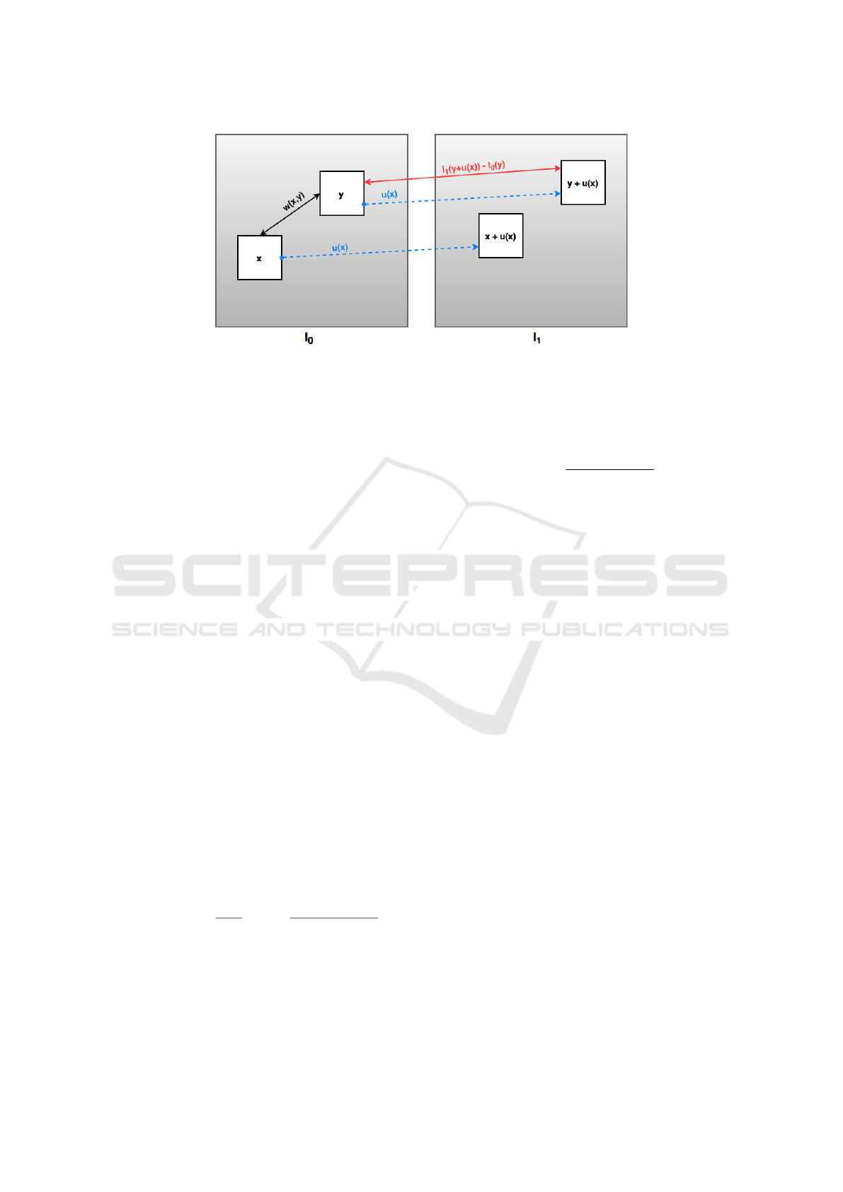
Figure 1: Graphical explanation of the Nonlocal Brightness Constancy Assumption (9). If a small window centered at x is
similar to a small window centered at y in the sense described by the support weights (10), then the displacement of x should
work for y. As a consequence, the intensity values I
1
(y + u(x)) and I
0
(y) should correspond to each other.
pixel color but the color of an entire window around.
Both aspects of weight definition makes (9) robust to
the existence of pixels with similar intensity values
but different displacements.
Finally, let us mention that the nonlocal bright-
ness constancy term is closely related to a bilateral
correction window and is in fact inspired by Yoon et
al. (Yoon and Kweon, 2006) and Xiao et al. (Xiao
et al., 2006), who used similar ideas for local match-
ing in stereo.
3.2 Nonlocal Matching Assumption
The second new-proposed term aims at replacing the
classic brightness constancy assumption. It uses a
weight family across the two images of the pair in or-
der to transfer window similarity to the displacement
field as follows:
Z
Ω
Z
Ω
ω(I
0
(x),I
1
(y))ψ(|I
1
(x + u(x)) −I
1
(y)|)dy dx.
(11)
Let us emphasize that the brightness constancy as-
sumption (2) cannot be obtained from (11) with any
weight distribution. Actually, the proposed term no
longer imposes a constraint on the motion trajectories
but a nonlocal self-similarity.
The weights in (11) measure the similarity be-
tween a patch centered at x in I
0
and another one cen-
tered at y in I
1
as follows:
ω(I
0
(x),I
1
(y)) =
1
Γ(x)
exp
−
d
ρ
(I
0
(x),I
1
(y))
h
2
c
,
(12a)
where the distance between patches is computed as
d
ρ
(I
0
(x),I
1
(y)) =
Z
Ω
G
ρ
(z)|I
0
(x + z) −I
1
(y + z)|
2
dz
(12b)
and the normalization factor is
Γ(x) =
Z
Ω
exp
−
d
ρ
(I
0
(x),I
1
(y))
h
2
c
dy. (12c)
Note that the difference between the weights defined
in (10) and those given in (12) is that the latter only
depend on the color similarity since the spatial close-
ness is not considered. This is because we do not want
the constraint (11) to be limited to small displace-
ments but to deal with pixels being relatively far from
each other, being the only limitation the linearization
of the numerical scheme if applicable.
Figure 2 illustrates the constraint defined in (11).
If pixels x in I
0
and y in I
1
are similar, then we can
expect the pixel in I
1
assigned to x by the flow field to
be similar to y. This is not a hard constraint since we
do not demand the pixel x to be matched with y, but
only to share a similar color.
The nonlocal matching assumption wants to intro-
duce patch comparison or block matching into the op-
tical flow variational formulation. Local block match-
ing methods compute motion by matching a small
window around any pixel in the first image with the
window in the second image minimizing a certain
cost. These methods fail when the window is not dis-
tinctive enough to be matched. This might be due
to the lack of texture inside the window but also to
the presence of several copies of the window in the
second image. In that case, which is known as the
aperture problem, local methods are not able to de-
cide among the different candidates. The use of the
weight configuration between patches of both images
in (12) permits introducing block matching as a soft
constraint into the energy. Therefore, (11) helps in
suppressing artifacts due to wrong motion estimations
and noise.
Nonlocal Regularizing Constraints in Variational Optical Flow
155
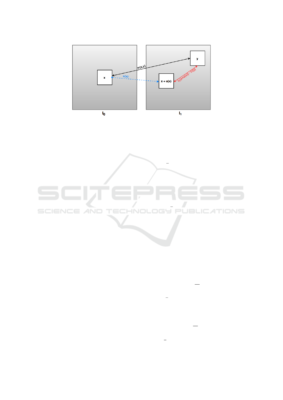
Figure 2: Graphical illustration of the Nonlocal Matching Assumption in (11). If a small window centered at x in I
0
is similar
to a small window centered at y in I
1
, as described by the support weights (12), then the displacement field should assign to x
a pixel in I
1
with an intensity value similar to y. As a consequence, the values I
1
(x + u(x)) and I
1
(y) should be similar.
3.3 The Energy Functionals
We specify now the full energy in the form (1).
Throughout this work, we employ quadratic func-
tions, i.e. ψ(s) = s
2
, to penalize the deviations from
the prescribed assumptions in (9) and (11). Even
though knowing the shortcomings of this choice,
which obviously may affect the quality of the results,
our aim is to compare the validity of the novel con-
straints with respect to the classical brightness con-
stancy assumption rather than pursuing the best pe-
nalization. The latter will be part of future work.
Let us notice that the proposed constraints are
nonlinear in u because of the warpings I
1
(y + u(x))
and I
1
(x + u(x)). We linearize both expressions using
Taylor expansions as follows:
g(u) := I
1
(y + u
0
(x)) −I
0
(y)
+ h∇I
1
(y + u
0
(x)),u(x) −u
0
(x)i,
f (u) := I
1
(x + u
0
(x)) −I
1
(y)
+ h∇I
1
(x + u
0
(x)),u(x) −u
0
(x)i,
(13)
with u
0
being a close approximation to u.
In addition to the data-fidelity terms, a critical part
in a variational model is the prior. The regularization
is responsible for the propagation of the flow from
boundaries to homogenous regions. This propagation
relies on the spatial coherence of natural images, thus
pixels belonging to the same object are supposed to
have almost the same flow. We incorporate the total
variation (Rudin et al., 1992) as regularization for the
two novel constraints.
Using (13), the final linearized nonlocal bright-
ness constancy energy is
E
l
γ
(u) :=
2
∑
m=1
Z
Ω
|∇u
m
(x)|dx
+
γ
2
Z
Ω
Z
Ω
ω(x,y,I
0
(x),I
0
(y))(g(u))
2
dy dx,
(14a)
while the linearized nonlocal matching energy is
E
l
δ
(u) :=
2
∑
m=1
Z
Ω
|∇u
m
(x)|dx
+
δ
2
Z
Ω
Z
Ω
ω(I
0
(x),I
1
(y))( f (u))
2
dy dx.
(14b)
4 NUMERICAL MINIMIZATION
4.1 Convex Relaxation of the Energies
Inspired by Zach et al. (Zach et al., 2007), we relax
the minimization of (14) by introducing an auxiliary
variable v which decouples the data and regularization
terms as
2
∑
m=1
Z
Ω
|∇u
m
(x)|dx +
1
2θ
ku −vk
2
+
γ
2
Z
Ω
Z
Ω
ω(x,y,I
0
(x),I
0
(y))(g(v))
2
dy dx
(15a)
and
2
∑
m=1
Z
Ω
|∇u
m
(x)|dx +
1
2θ
ku −vk
2
+
δ
2
Z
Ω
Z
Ω
ω(I
0
(x),I
1
(y))( f (v))
2
dy dx.
(15b)
VISAPP 2017 - International Conference on Computer Vision Theory and Applications
156

Therefore, one can compute the solution by alter-
nating minimizations:
i) Fixed v, solving (15) with respect to u is a TV-
based problem, the solution of which is computed
using Chambolle’s projection algorithm (Cham-
bolle, 2004).
ii) Fixed u, the minimizer of (15) with respect to v
can be computed explicitly due to the quadratic
penalization in the data-fidelity energy terms.
4.2 Computation of the Weights
For computational purposes, the nonlocal interaction
is limited to pixels at a certain distance, the so-called
research window. More precisely, given a parameter
ν > 0, we redefine the weights (10) and (12) as
ω(x,y,I
0
(x),I
0
(y)) =
1
Γ(x)
exp
−
kx −yk
2
h
2
s
·
·exp
−
1
h
2
c
∑
z∈N
0
|I
0
(x + z) −I
0
(y + z)|
2
!
(16)
and
ω(I
0
(x),I
1
(y)) =
1
Γ(x)
·
·exp
−
1
h
2
c
∑
z∈N
0
|I
0
(x + z) −I
1
(y + z)|
2
!
(17)
if kx −yk
∞
≤ ν, and ω ≡ 0 otherwise. Here, N
0
is a
rectangular window centered at 0, the so-called com-
parison window. The Gaussian kernel G
ρ
introduced
in (10) and (12) is not considered in practice as it
is only necessary when the size of the windows in-
crease considerably. After all, the weight distribution
is commonly sparse.
4.3 Coarse-to-Fine Approach
A problem that arises with the linearizations per-
formed in (13) is how to determine the value of u
0
in
order to allow large disparities between images. We
use a coarse-to-fine scheme to reduce the distance be-
tween the objects in the scene. Furthermore, in each
scale, u
0
is iteratively refined to assure convergence.
We employ image pyramids of 5 scales with a sub-
sampling factor of 2. The images are smoothed with
a Gaussian kernel of standard deviation 1.04 before
subsampling. Beginning with the coarsest level, we
solve (15) at each scale of the pyramid and propagate
the solution to the next one as u
s−1
(x) = 2u
s
(0.5x).
Every intermediate solution is used as the initializa-
tion in the following scale. In each scale, we intro-
duce 5 intermediate steps to update u
0
and warp I
1
.
At the beginning of a new scale, v is initialized with
u and, at the coarsest one, u starts with 0.
The displacement to be detected must be small
at the coarsest scale. In this respect, one drawback
of the pyramidal approach is that the method can-
not estimate the motion of small objects undergoing
large displacements, since these may disappear in the
coarsest scales. However, let us emphasize that this is
not a limitation of the new-proposed constraints, but
it is a matter of the linearization and the optimization
strategy we have chosen.
Spatial image and flow derivatives are discretized
using central differences and forward differences, re-
spectively, with Neumann boundary conditions. Fur-
thermore, we use bicubic interpolation to warp the
image I
1
and its derivatives. At each warp, the min-
imization procedure alternates one step of the fixed-
point scheme to update u (Chambolle, 2004) with the
explicit computation of v. As stopping criterion we
use a tolerance value of 10
−6
for the relative error be-
tween two consecutive iterations. Anyway, we stop
the algorithm after 1000 iterations even if the toler-
ance is not reached.
The optical flow is computed on the grayscale
images and the sizes of the research and compari-
son windows used in the support weights are fixed to
21 ×21 and 7 ×7 pixels, respectively. Furthermore,
we integrate a median filter of size 7 ×7 into the nu-
merical scheme to increase the robustness to sampling
artifacts in the image data (Wedel et al., 2009). For all
models under comparison, this filtering step is applied
after each warp.
Finally, let us mention that the computational
costs of the two new-proposed methods given in (15)
are equivalent to the computational cost of the clas-
sical TV-L2 method, that is, the one penalizing the
linearized counterpart of the brightness constancy as-
sumption with the Euclidean norm. Indeed, we have
only to perform an extra weight computation at the
beginning of each scale of the multi-resolution pyra-
mid. Since this might be easily parallelized, the in-
crease in running time is negligible.
5 EXPERIMENTAL RESULTS
This section aims at comparing the two novel data
terms with the classic brightness constancy assump-
tion. We evaluate the methods with the Middlebury
benchmark (Barker et al., 2011) with known ground
truth, so that we can determine the optimal param-
Nonlocal Regularizing Constraints in Variational Optical Flow
157
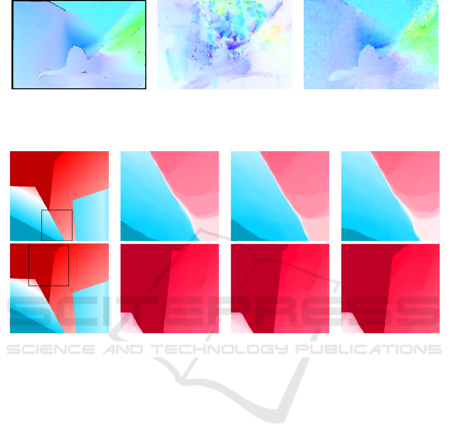
Reference Classical Constraint (3) Nonlocal Constraint (9)
Figure 3: Optical flow estimation without regularization. For the classic linearized constraint (3) we added a TV regularization
term limiting its role as much as possible. While (3) leads to an unstable flow, the nonlocal brightness constancy assumption
(9) permits the computation of an admissible solution without any prior.
Reference Classic energy E
l
γ
E
l
δ
Figure 4: Reference and obtained flow fields for the “Venus” sequence. The AEPE are 0.313, 0.309, and 0.310 for the classic,
E
l
γ
, and E
l
δ
energies, respectively.
eters in terms of the lowest average end-point error
(AEPE). The color scheme used in all experiments to
represent the orientation and magnitude of the optical
flow is the same as that of Barker et al. (Barker et al.,
2011). In order to fairly compare all variational mod-
els, we use a numerical scheme similar to (15) for the
model based on the brightness constancy assumption
(2), but penalizing its linearized counterpart, given in
(3), with the L
2
norm.
It is well known that it is not possible to determine
the flow from (3) since the number of parameters to be
estimated is larger than the number of linearly inde-
pendent equations. However, the linearized nonlocal
brightness constancy constraint (9) allows us to get
an explicit solution for the motion without any prior.
Figure 3 displays the obtained flows in both cases –
since (3) is ill-posed, we added the TV regularization
but reducing its role as much as possible. We observe
that, as expected, the classical constraint leads to an
unstable flow as the regularization vanishes. The con-
straint (9) is able to give an admissible result without
any prior instead.
Figures 4 and 5 provide the flow fields obtained
for the “Venus” and “Rubberwhale” sequences, re-
spectively. We also display the corresponding AEPE
values in order to numerically compare the results
with the ground truth. We have excluded from this
measure the pixels in the occlusions, which are avail-
able for the Middlebury benchmark. The AEPE val-
ues were computed for the whole image and not only
for the close-ups showed in the figures. While there
is hardly any visual difference between the flow fields
estimated by the classic energy and E
l
δ
in the first row
of Figure 4, the latter is convincingly better in the
close-ups from the second row. Indeed, E
l
δ
is able
to correctly estimate the flow at the boundaries of the
objects – see the slope at the top of these images. On
the other hand, the nonlocal brightness constancy as-
sumption in E
l
γ
identifies the gap in the middle of the
Venus image better than the others, as highlighted in
the close-ups from the first row. Similar behavior of
E
l
γ
can be observed in the Rubberwhale sequence. In
VISAPP 2017 - International Conference on Computer Vision Theory and Applications
158
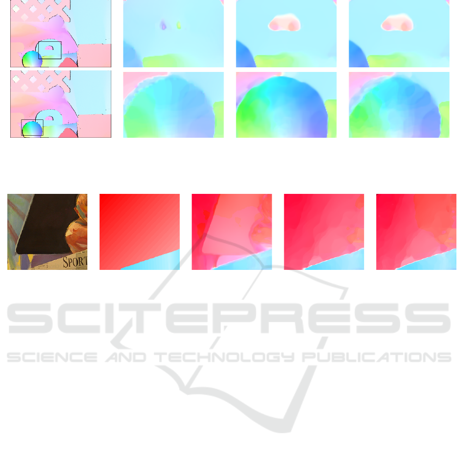
Reference Classic energy E
l
γ
E
l
δ
Figure 5: Reference and obtained flow fields for the “Rubberwhale” sequence. The AEPE are 0.209, 0.154, and 0.199 for the
classic, E
l
γ
, and E
l
δ
energies, respectively.
Frame Reference NLTV E
l
γ
E
l
δ
Figure 6: Source frame, reference and obtained flow fields for the “Venus” sequence. The classic optical flow constraint (3)
is regularized using nonlocal strategies (NLTV). Observe that NLTV copies the geometry and texture of the source frame into
the estimated flow, which does not happen with the nonlocal constraints E
l
γ
and E
l
δ
.
this case, both E
l
γ
and E
l
δ
detect the hole in the let-
ter ‘e’, which is not the case with the classic con-
straint. The results in the second row of Figure 5 show
that E
l
γ
provides the best visual and numerical per-
formance. In the end, the two nonlocal regularizing
data terms show a significantly discriminative poten-
tial when compared with the classic energy. Further-
more E
l
δ
is proved to replace the brightness constancy
assumption efficiently without matching points along
the trajectory.
We finally compare the two new-proposed non-
local constraints with the nonlocal regularization (8)
used as prior jointly with the optical flow constraint
given in (3) (Werlberger et al., 2010; Ranftl et al.,
2014). Figure 6 displays close-ups of the estimated
motion for the Venus sequence. We observe that the
nonlocal regularization forces the geometry and tex-
ture of the image into the flow field, identifying wrong
motion patterns. On the contrary, the proposed data
terms use the image geometry correctly to regularize
the flow and better locate flow discontinuities.
6 CONCLUSIONS
In this paper, we have introduced two nonlocal con-
straints for optical flow estimation. The image geom-
etry is used to propose regularized data-fidelity terms
making the flow computation more robust and able
to better locate motion discontinuities. The experi-
mental results have illustrated their superiority with
respect to the classic brightness constancy assump-
tion. The results also demonstrate that image self-
similarity can be better taken advantage of in the data-
fidelity terms than in the regularization prior. For the
moment, we limited ourselves to illustrate the perfor-
mance of each term separately, the combination of
them will be object of future research.
The limitations of this work are in the optimiza-
tion strategy rather than in the models themselves.
We have linearized the constraints, forcing us to em-
bed the optimization in a coarse-to-fine warping. Fu-
ture work will mainly concentrate on postponing the
linearization to the numerical scheme and using the
nonlinear formulations directly, which will require a
careful minimization strategy.
Nonlocal Regularizing Constraints in Variational Optical Flow
159

ACKNOWLEDGEMENTS
The authors were supported by the Ministerio de
Ciencia e Innovaci
´
on of the Spanish Government un-
der grant TIN2014-53772-R. During this work, J. Du-
ran had a fellowship of the Obra Social La Caixa.
REFERENCES
Alvarez, L., Deriche, R., Papadopoulo, T., and S
´
anchez, J.
(2002). Symmetrical dense optical flow estimation
with occlusions detection. In Proc. European Conf.
Computer Vision (ECCV), volume 2350 of Lecture
Notes in Comp. Sci., pages 721–735, Copenhagen,
Denmark.
Alvarez, L., Weickert, J., and S
´
anchez, J. (2000). Reliable
estimation of dense optical flow fields with large dis-
placements. Int. J. Comput. Vis., 39(1):41–56.
Barker, S., Scharstein, D., Lewis, J., Roth, S., Black, M.,
and Szeliski, R. (2011). A database and evaluaton
methodology for optical flow. Int. J. Comput. Vis.,
92(1):1–31.
Black, M. and Anandan, P. (1996). The robust estimation of
multiple motions: Parametric and piecewise smooth
flow fields. Comput. Vis. Image Underst., 63(1):75–
104.
Brox, T., Bruhn, A., Papenberg, N., and Weickert, J. (2004).
High accuracy optical flow estimation based on a the-
ory for warping. In Proc. European Conf. Com-
puter Vision (ECCV), volume 3024 of Lecture Notes
in Comp. Sci., pages 25–36, Prague, Czech Republic.
Brox, T. and Malik, J. (2011). Large displacement opti-
cal flow: Descriptor matching in variational motion
estimation. IEEE Trans. Pattern Anal. Mach. Intell.,
33(3):500–513.
Bruhn, A., Weickert, J., and Schn
¨
orr, C. (2005). Lu-
cas/Kanade meets Horn/Schunck: Combining local
and global optic flow methods. Int. J. Comput. Vis.,
61(3):211–231.
Buades, A., Coll, B., and Morel, J.-M. (2005). A review of
image denoising algorithms, with a new one. SIAM
Multiscale Model. Simul., 4(2):490–530.
Chambolle, A. (2004). An algorithm for total variation
minimization and applications. J Math. Imaging Vis.,
20(1–2):89–97.
Horn, B. and Schunck, B. (1981). Determining optical flow.
In Technical Symposium East, pages 319–331. Inter-
national Society for Optics and Photonics.
Kennedy, R. and Taylor, C. (2015). Optical flow with
geometric occlusion estimation and fusion of multi-
ple frames. In Proc. Int. Conf. Energy Minimization
Methods in Computer Vision and Pattern Recogni-
tion (EMMCVPR), volume 8932 of Lecture Notes in
Comp. Sci., pages 364–377, Hong Kong.
Lowe, D. (2004). Distinctive image features from scale-
invariant keypoints. Int. J. Comput. Vis., 60(2):91–
110.
Lucas, B. and Kanade, T. (1981). An iterative image regis-
tration technique with an application to stereo vision.
In Proc. Int. Joint Conf. Artificial Intelligence, pages
674–679, Vancouver, BC, Canada.
M
´
emin, E. and P
´
erez, P. (1998). Dense estimation and
object-based segmentation of the optical flow with
robust techniques. IEEE Trans. Image Process.,
7(5):703–719.
Mileva, Y., Bruhn, A., and Weickert, J. (2007).
Illumination-robust variational optical flow with pho-
tometric invariants. In Proc. DAGM Symposium on
Pattern Recognition, volume 4713 of Lecture Notes in
Comp. Sci., pages 152–162, Heidelberg, Germany.
Nagel, H.-H. and Enkelmann, W. (1986). An investigation
of smoothness constraints for the estimation of dis-
placement vector fields from image sequences. IEEE
Trans. Pattern Anal. Mach. Intell., 8(5):565–593.
Papenberg, N., Bruhn, A., Brox, T., Didas, S., and Weick-
ert, J. (2006). Highly accurate optic flow computation
with theoretically justified warping. Int. J. Comput.
Vis., 67(2):141–158.
Ranftl, R., Bredies, K., and Pock, T. (2014). Non-local total
generalized variation for optical flow estimation. In
Proc. European Conf. Computer Vision (ECCV), vol-
ume 8698 of Lecture Notes in Comp. Sci., pages 439–
454, Zurich, Switzerland. Springer Berlin Heidelberg.
Rudin, L., Osher, S., and Fatemi, E. (1992). Nonlinear total
variation based noise removal algorithms. Physica D,
60:259–268.
Steinbr
¨
ucker, F., Pock, T., and Cremers, D. (2009). Large
displacement optical flow computation without warp-
ing. In Proc. IEEE Int. Conf. Computer Vision (ICCV),
pages 1609–1614, Kyoto, Japan.
Trobin, W., Pock, T., Cremers, D., and Bischof, H. (2008).
An unbiased second-order prior for high-accuracy
motion estimation. In Proc. DAGM Symposium on
Pattern Recognition, volume 5096 of Lecture Notes
in Comp. Sci., pages 396–405, Munich, Germany.
Vogel, C., Roth, S., and Schindler, K. (2013). An eval-
uation of data costs for optical flow. In Proc. Ger-
man Conference Pattern Recognition (GCPR), vol-
ume 8142 of Lecture Notes in Comp. Sci., pages 343–
353, Saarbr
¨
ucken, Germany.
Wedel, A., Pock, T., Zach, C., Cremers, D., and Bischof,
H. (2009). An improved algorithm for TV-L1 optical
flow. In Proc. Statistical and Geometrical Approached
to Visual Motion Analysis, volume 5604 of Lecture
Notes in Comp. Sci., pages 23–45, Dagstuhl Castle,
Germany.
Werlberger, M., Pock, T., and Bischof, H. (2010). Mo-
tion estimation with non-local total variation regular-
ization. In Proc. IEEE Conf. Computer Vision and
Pattern Recognition (CVPR), pages 2464–2471, San
Francisco, CA, USA.
Werlberger, M., Trobin, W., Pock, T., Bischof, H., Wedel,
A., and Cremers, D. (2009). Anisotropic Huber-L1
optical flow. In Proc. British Machine Vision Confer-
ence (BMVC), pages 108.1–108.11, London, UK.
Xiao, J., Cheng, H., Sawhney, H., Rao, C., and Isnardi,
M. (2006). Bilateral filtering-based optical flow es-
VISAPP 2017 - International Conference on Computer Vision Theory and Applications
160

timation with occlusion detection. In Proc. European
Conf. Computer Vision (ECCV), volume 3951 of Lec-
ture Notes in Comp. Sci., pages 211–224, Graz, Aus-
tria.
Yoon, K. and Kweon, I. (2006). Adaptive support-weight
approach for correspondece search. IEEE Trans. Pat-
tern Anal. Mach. Intell., 28(4):650–656.
Zach, C., Pock, T., and Bischof, H. (2007). A duality based
approach for realtime TV-L1 optical flow. In Proc.
DAGM Symposium on Pattern Recognition, volume
4713 of Lecture Notes in Comp. Sci., pages 214–223,
Heidelberg, Germany.
Zimmer, H., Bruhn, A., and Weickert, J. (2011). Optic flow
in harmony. Int. J. Comput. Vis., 93(3):368–388.
Zimmer, H., Bruhn, A., Weickert, J., Valgaerts, L., Salgado,
A., Rosenhahn, B., and Seidel, H.-P. (2009). Com-
plementary optic flow. In Proc. Int. Conf. Energy
Minimization Methods in Computer Vision and Pat-
tern Recognition (EMMCVPR), volume 5681 of Lec-
ture Notes in Comp. Sci., pages 207–220, Bonn, Ger-
many.
Nonlocal Regularizing Constraints in Variational Optical Flow
161
