Regularised Energy Model
for Robust Monocular Ego-motion Estimation
Hsiang-Jen Chien and Reinhard Klette
School of Engineering, Computer and Mathematical Sciences,
Auckland University of Technology, Auckland, New Zealand
Keywords:
Visual Odometry, Camera Motion Recovery, Perspective-n-points Problem, Nonlinear Energy Minimisation.
Abstract:
For two decades, ego-motion estimation is an actively developing topic in computer vision and robotics. The
principle of existing motion estimation techniques relies on the minimisation of an energy function based on
re-projection errors. In this paper we augment such an energy function by introducing an epipolar-geometry-
derived regularisation term. The experiments prove that, by taking soft constraints into account, a more reliable
motion estimation is achieved. It also shows that the implementation presented in this paper is able to achieve
a remarkable accuracy comparative to the stereo vision approaches, with an overall drift maintained under 2%
over hundreds of metres.
1 INTRODUCTION
Recovering camera motion from imagery data is one
of the fundamental problems in computer vision.
Image-based motion estimation provides a comple-
mentary solution to GPS-engaged positioning sys-
tems which might fail in close-range (e.g. indoor) en-
vironments or due to any circumstances without clear
satellite signals. A variety of techniques can be found
in a number of applications in the context of simulta-
neously localisation and mapping (SLAM) (Konolige
et al., 2008), structure from motion (SfM), or visual
odometry (VO) (Scaramuzza and Fraundorfer, 2011).
The estimation of camera motion can be achieved
in different ways, up to the availability of inter-frame
point correspondences. In the case of ToF or RGB-D
cameras where the pixel depths are available, the rel-
ative pose of the sensor between two different frames
can be derived using 3D-to-3D correspondences by
means of rigid body registration (Hu et al., 2012). It is
a more general case where the 3D coordinates of pix-
els are known only in the previous frame with their
locations observed in the current frame. In such a
case the ego-motion is estimated from 3D-to-2D cor-
respondences, and the minimisation of the deviations
of the projected 3D coordinates from the observed 2D
locations has been proven to be the golden standard
solution to the ego-motion estimation problem (En-
gels et al., 2006).
In this paper we provide a quick review for the un-
derlying mathematical models of the monocular ego-
motion estimation problem. Based on these mod-
els, we propose an augmented energy function that
regularises the iterative adjustment of estimated ego-
motion by taking epipolar constraints into account.
The paper is organised as follows. In Section 2
we provide a literature review on mathematical foun-
dations of the monocular ego-motion estimation prob-
lem. In Section 3 a revised energy model is proposed
which is then verified by the experiments reported in
Section 4. We conclude this paper in Section 5.
2 MONOCULAR EGO-MOTION
We review the common process by starting with the
theory, and ending with comments on implementa-
tion.
Theory. Following the pinhole camera projection
model, a 3D point P = (x, y,z) is projected into a pixel
location (u, v) in the image plane by


u
v
1


∼


f
u
0 u
c
0
0 f
v
v
c
0
0 0 1 0





x
y
z
1



= (K0)



x
y
z
1



(1)
where the upper 3× 3 triangular matrix K is the cam-
era matrix modelled by the intrinsic parameters of the
Chien H. and Klette R.
Regularised Energy Model for Robust Monocular Ego-motion Estimation.
DOI: 10.5220/0006100303610368
In Proceedings of the 12th International Joint Conference on Computer Vision, Imaging and Computer Graphics Theory and Applications (VISIGRAPP 2017), pages 361-368
ISBN: 978-989-758-227-1
Copyright
c
 2017 by SCITEPRESS – Science and Technology Publications, Lda. All rights reserved
361

camera including focal lengths f
u
and f
v
, and the im-
age centre or principle point (u
c
, v
c
). By ∼ we denote
projective equality (i.e. equality up to a scale).
As the camera moves to a new position, the same
point P, if it remains stationary, is observed at a dif-
ferent pixel location. The movement of the camera in-
troduces a new coordinate system which can be mod-
elled by an Euclidean transformation with respect to
the previous frame. Let (R t) be such a transforma-
tion, where R ∈ SO(3) is the rotation matrix, and
t ∈ R
3
is the translation vector. The new projection
of point P is found by


u
0
v
0
1


∼ K

R t




x
y
z
1



(2)
3D-to-2D ego-motion estimation algorithms rely on
the principle that, given sufficiently many observa-
tions (x, y, z) ↔ (u
0
, v
0
), it is possible to determine
the unknown transformation (R t). The estimation
of such transformations is known as the perspective-
from-n-points (PnP) problem (Lepetit et al., 2009).
A linear approach treats the projection as a general
linear transform controlled by the 3-by-4 projection
matrix P = K

R t

. For each observation (x, y, z) ↔
(u
0
, v
0
), two linear constraints are obtained as follows:


−u
0
x −u
0
y −u
0
z
A
−v
0
x −v
0
y −v
0
z




P
>
1
P
>
2
P
>
3


= 1 (3)
where P
i
denotes the i-th row of the projection matrix
P, and
A =

x y z 0 0
0 0 0 x y

(4)
Having six world-image correspondences, a linear
system of twelve unknowns can be constructed. If the
observations are linearly independent then the matrix
P can be calculated, allowing one in turn to use the
calibrated camera matrix K to recover the motion by

R t

= K
−>
P (5)
In practice more than six correspondences are used
to construct an over-determined linear system, and a
least-squares-solution yields a more robust solution.
This strategy is known as the direct linear transform
(DLT) method.
As an Euclidean transformation essentially has six
degrees of freedom (DoF) while there are twelve un-
knowns in P, the recovered rotation matrix R is not
guaranteed to be a valid element in SO(3) due to over-
parameterization. Furthermore, the minimised alge-
braic errors, subject to Eq. (3), lack of geometric in-
terpretation. To address these issues, a nonlinear ad-
justment strategy is usually carried out following the
linear estimation step.
Assuming that the 3D measurement noise follows
a Gaussian model, the maximum-likelihood estima-
tion (MLE) of (R t) is achieved by a minimisation of
the sum-of-squares of the reprojection error:
φ
R
(R, t) =
∑
i



(u
0
i
, v
0
i
)
>
− π
K
[R(x
i
, y
i
, z
i
)
>
+ t]



2
Σ
i
(6)
where π
K
: R
3
→ R
2
is the projection function that
maps a 3D point into the projective space P
2
using
the camera matrix K. It also converts the resulting
homogeneous coordinates into a Cartesian plane. By
Σ
i
we denote the 2 × 2 error covariance matrix of the
i-th-point correspondence.
As Eq. (6) cannot be solved in any closed form,
one may adopt a nonlinear least-squares minimiser,
say the Levenberg-Marquardt algorithm (Levenberg,
1944), to minimise the energy function, starting with
the solution found using the DLT estimation as an ini-
tial guess.
Motion without 3D Prior. For a monocular vision
system, 3D coordinates (x, y, z) might not be available
as a prior. In this case, the motion of the camera can
still be recovered from epipolar conditions but where
the scale of t remains undetermined. Without loss of
generality, we assume that ktk = 1 in the following
context. Let (u, v) ↔ (u
0
, v
0
) be a 2D-to-2D corre-
spondence. It follows that


u
0
v
0
1


>
K
−>
[t]
×
RK
−1


u
v
1


= 0 (7)
where
[t]
×
=


0 −t
z
t
y
t
z
0 −t
x
−t
y
t
x
0


(8)
denotes the skew-symmetric form of t = (t
x
,t
y
,t
z
)
>
.
Equation (7) is the well-known epipolar condition,
and the matrix E = [t]
×
R is called the essential ma-
trix.
Among a variety of essential matrix recovery tech-
niques, the eight-point algorithm is a popular choice.
The method first estimates the fundamental matrix
F = K
−>
EK
−1
using at least eight point correspon-
dences. For each correspondence (u, v) ↔ (u
0
, v
0
), a
homogeneous constraint is introduced by Eq. (7) as
follows:
uu
0
f
11
+ vu
0
f
12
+ u
0
f
13
+ uv
0
f
21
+ vv
0
f
22
+v
0
f
23
+ u f
31
+ v f
32
+ f
33
= 0 (9)
where f
i j
denotes an element of the fundamental ma-
trix. By means of linear algebra techniques, all the
nine elements of the fundamental matrix can be de-
termined up to a scale using at least eight constraints.
VISAPP 2017 - International Conference on Computer Vision Theory and Applications
362

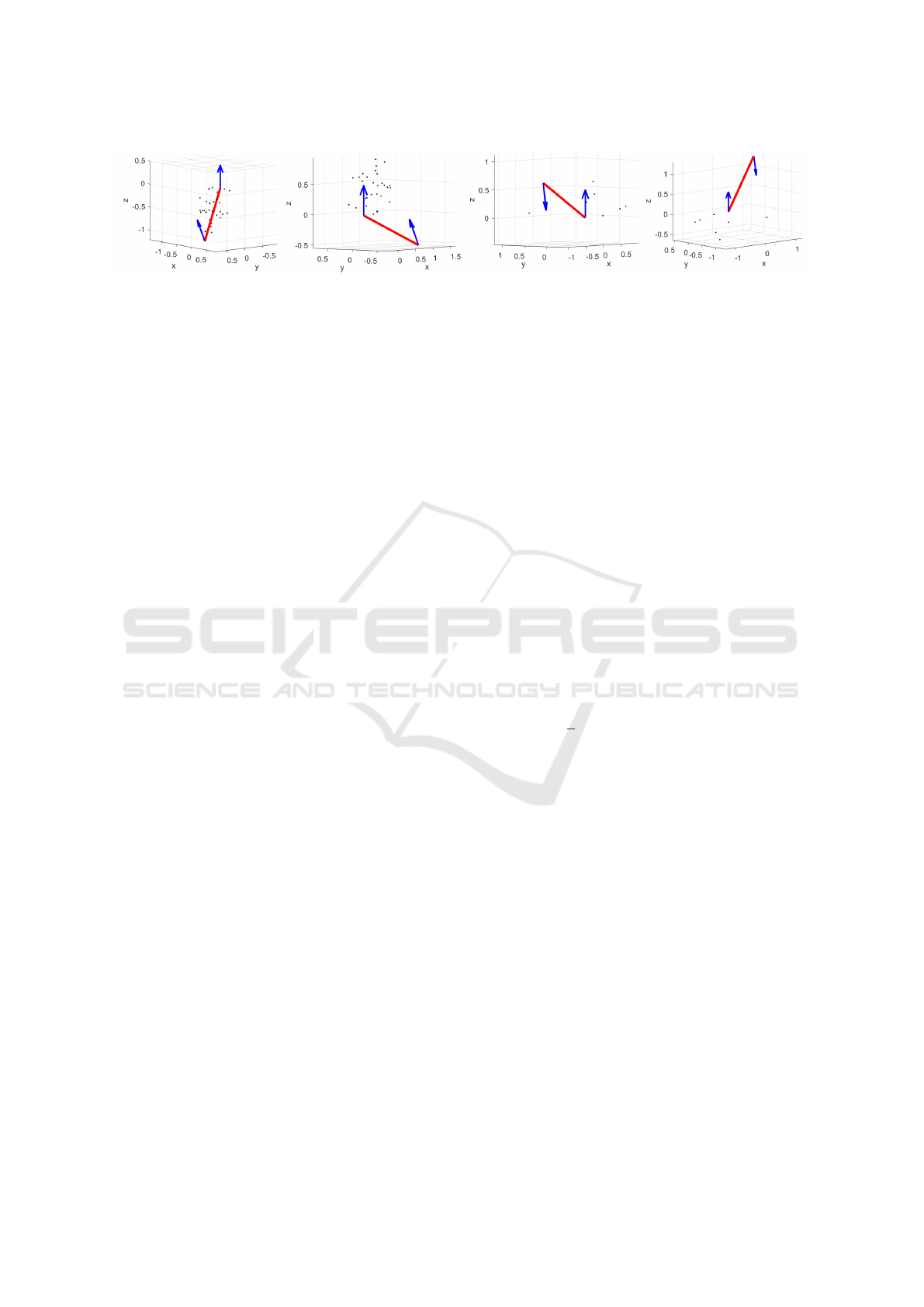
Figure 1: An example of four possible ego-motion estimates from essential matrix decomposition. Only the second to the
leftmost solution shows a valid geometric configuration, where all the triangulated 3D points lie in front of both cameras.
According to E = K
>
FK, one may obtain the es-
sential matrix from the solved fundamental matrix.
The motion, denoted by R and t, can be extracted
from a calculated essential matrix E. One may com-
pute a singular value decomposition (SVD)
E = UDV
>
(10)
of matrix E where U and V are 3 × 3 orthonormal
matrices, and D = diag(1, 1, 0) is a diagonal matrix
having a 1 as the first and second diagonal element,
and 0 as the third (due to the rank deficiency of E).
By introducing two matrices
Z =


0 ±1 0
∓1 0 0
0 0 0


, W =


0 ∓1 0
±1 0 0
0 0 ±1


(11)
and based on D = ZW and U
>
U = I, one may now
rewrite Eq. (10) as follows:
E = UZU
>
UWV
>
(12)
It is verified that S = UZU
>
is a skew-symmetric ma-
trix, and R
0
= UWV
>
is an orthonormal matrix. Fol-
lowing the definition E = [t]
×
R = SR
0
, the rotation
matrix R and the unit translation vector t are instantly
found.
Due to the sign ambiguity of Z and W, there are
four possible solutions. As described in the next sec-
tion, the best candidate is decided by applying a tri-
angulation method on (u, v) ↔ (u
0
, v
0
), and checking
the number of the resulting points that fall in front of
the cameras to select the best candidate. In the non-
singular case, only one candidate gives a valid geo-
metric setup. Figure 1 depicts an example of all the
four possible solutions.
Triangulation. Triangulation is the process of com-
puting 3D coordinates (x, y, z) given an inter-frame 2D
point correspondence (u, v) ↔ (u
0
, v
0
), and the cam-
era’s motion (R t), in the context of monocular vision.
As in a practical case, the back-projected rays can-
not be expected to meet at an exact point in 3D space,
an error metric has to be adopted. The triangulation
procedure then looks for the best solution (x, y, z) that
minimises the defined error. A reasonable choice is
to find the 3D point which has the shortest Euclidean
distances to both of the back-projected rays. In such
a case, the error is defined as follows with respect to
free parameters k, k
0
∈ R
+
:
δ
mid
(k, k
0
) = kka − (k
0
a
0
+ c
0
)k
2
(13)
where a = K
−1
(u, v,1)
>
and a
0
= R
>
K
−1
(u
0
, v
0
, 1)
>
are the directional vectors of the back-projected rays,
and c
0
= −R
>
t is the new camera centre (i.e. principle
point) as seen in the last position’s coordinate system.
The minimum of Eq. (13) can be found by calcu-
lating the least-squares solution of the following lin-
ear system:

a −a
0


k
k
0

= A

k
k
0

= c
0
(14)
The resulting values k and k
0
denote two points on
each of the back-projected rays at the shortest mu-
tual distance in 3D space, and the midpoint of them
is therefore the optimal solution subject to the defined
error metric. In particular, we have that
(x, y, z)
>
=
1
2


a a
0

(A
>
A)
−1
A
>
+ I

c
0
(15)
This approach is known as mid-point triangulation.
If the noise of the correspondence (u,v) ↔ (u
0
, v
0
)
is believed to be Gaussian, it is proper to alternatively
adopt the so-called optimal triangulation method.
The MLE of the triangulated coordinates is achieved
by minimising
δ
optimal
(
ˆ
x,
ˆ
x
0
) = k(u, v)
>
−
ˆ
xk
2
Σ
+ k(u
0
, v
0
)
>
−
ˆ
x
0
k
2
Σ
(16)
subject to the epipolar constraint
ˆ
x
0>
F
ˆ
x = 0, with
ˆ
x =
π
K

(x, y, z)
>

and
ˆ
x
0
= π
K

R · (x, y,z)
>
+ t

being the
projections of the estimated 3D point.
Equation (16) poses a quadratically-constrained
minimisation problem which, unfortunately, has no
close-form solution. In recent years, several strate-
gies have been developed to iteratively approach an
optimal solution (see (Wu et al., 2011) for an exam-
ple.)
Implementation. Based on the models described
so far, monocular vision ego-motion estimation al-
gorithms have been designed. To acquire inter-frame
Regularised Energy Model for Robust Monocular Ego-motion Estimation
363

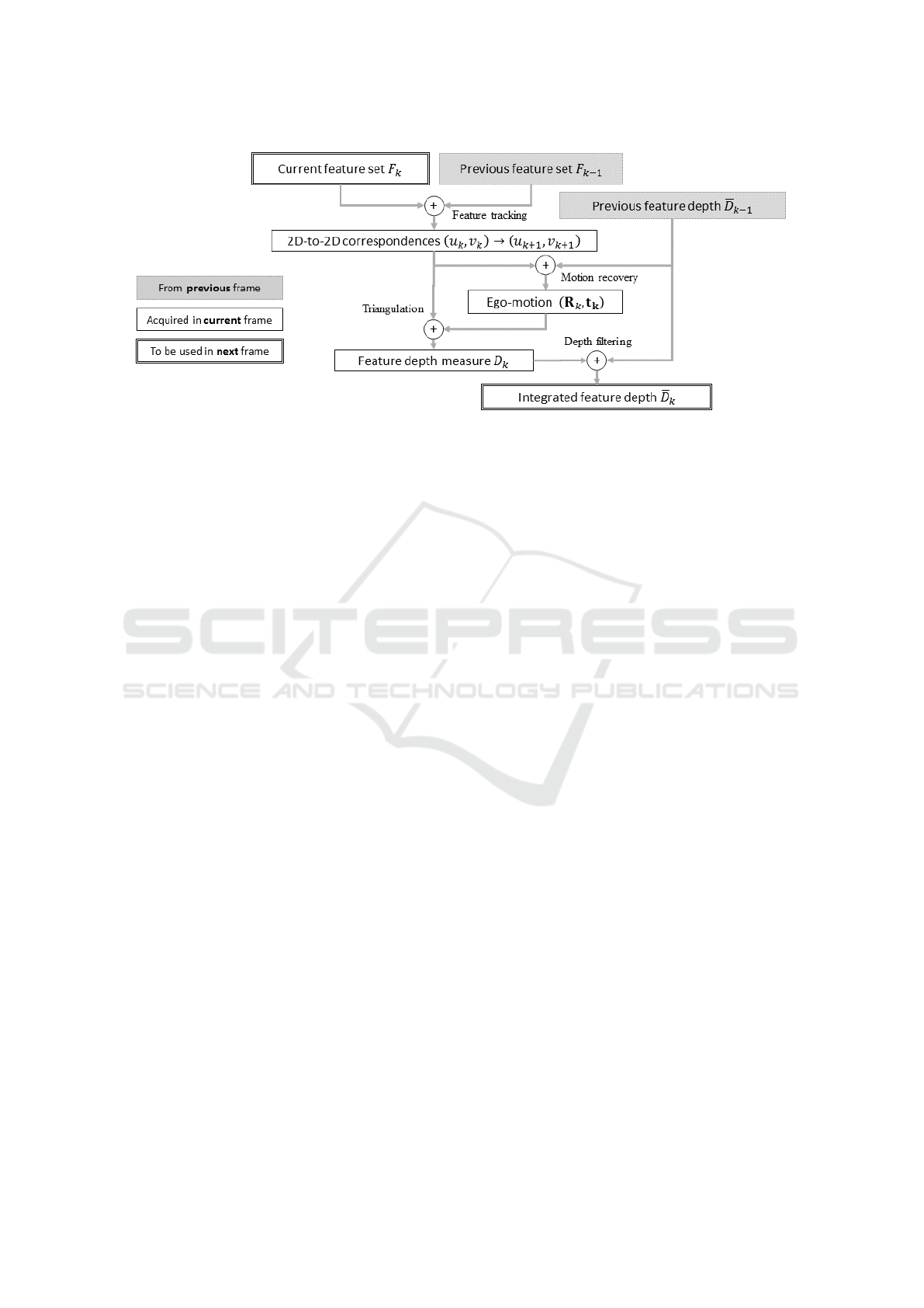
Figure 2: The pipeline of an implemented ego-motion estimator, based on the models described in Section 2.
pixel correspondences, two approaches might be con-
sidered. The first one is using all the intensities to
match image blocks and produce dense correspon-
dences; this is known as the patch-based technique
(e.g.(Forster et al., 2014)). Alternatively, one may
compare fewer but characteristic representative re-
gions to establish sparse correspondences; this is
known as the feature-based approach. In this section
we outline an implementation based on the later tech-
nique.
In order to estimate the motion of a camera, be-
tween frame k and k + 1, we first detect feature
point sets F
k
and F
k+1
, respectively, from these two
frames. The feature vectors (or feature descriptors) of
these sets are then computed and matched in a high-
dimensional feature space R
n
(usually n > 50), by
means of the Euclidean metric.
As the 3D information is not available initially, a
bootstrapping technique is required to initiate the ego-
motion estimation process. This can be done by ap-
plying the techniques described in Section 2 on the
matched pixel correspondences in frames k = 0 and
k = 1. The resulting motion (R
1
t
1
) can then be used
to triangulate the 3D coordinates of the i-th pixel cor-
respondence (u
i,0
, v
i,0
) ↔ (u
i,1
, v
i,1
).
As the camera moves to the next position for
frame k = 2, the previously triangulated 3D coordi-
nates are used with the newly discovered pixel corre-
spondences to recover the motion, based on the linear
initialisation and non-linear minimisation models in-
troduced in Section 2.
It is common to see a scene point involved in the
ego-motion estimation in multiple frames through a
sequence. This results in multiple depth estimations
for the same point. Due to the error of the estimated
ego-motion, the error of feature matching, and the nu-
merical stability of the adopted triangulation method,
calculated depths differ for a considered scene point,
once aligned to the same coordinate system.
A depth filtering technique, in this case, may be
used to fuse these measures and yield a more robust
result. The recently proposed multi-frame feature in-
tegration (MFI) technique (Badino et al., 2013) and
Kalman filter-based solutions (e.g. (Geng et al., 2015;
Klette, 2014; Morales and Klette, 2013; Vaudrey et
al., 2008)) are good choices.
Based on the ideas presented in this section, one
may implement an ego-motion estimator which fol-
lows the pipeline illustrated by Figure 2. We leave the
discussion regarding the depth integration step to the
next section.
3 PROPOSED METHOD
In this section we introduce a regularised energy
model to achieve more robust ego-motion recovery.
An iterative depth-integration technique is also pre-
sented to further improve the performance of the mo-
tion estimation process, as more data are gathered
through the sequence.
Regularised Energy Model. The idea of regulari-
sation is to use not only 3D-to-2D point correspon-
dences (x
k
, y
k
, z
k
) ↔ (u
k+1
, v
k+1
) but also 2D-to-2D
mappings (u
k
, v
k
) ↔ (u
k+1
, v
k+1
) to evaluate a motion
hypothesis (R
k
t
k
) from frame k to k + 1.
The decision of an Euclidean transform (
ˆ
R
ˆ
t) be-
tween two views immediately instantiates an epipolar
geometry, encoded by the fundamental matrix
ˆ
F = K
−>
[
ˆ
t]
×
ˆ
RK
−1
(17)
Intuitively one may take into account the deviation of
the observed correspondences from the epipolar con-
straint imposed by
ˆ
F during the energy minimisation
VISAPP 2017 - International Conference on Computer Vision Theory and Applications
364

process. That is, in addition to the reprojection error,
the minimisation now also considers the regularisa-
tion term
φ
E
(
ˆ
R,
ˆ
t) =
∑
i

x
0
>
i,k+1
·
ˆ
F · x
i,k

2
(18)
where x
i,k
= (u
i,k
, v
i,k
, 1)
>
. Such modelling, however,
is found biased and tends to move the epipole toward
the image centre, as the algebraic term x
0>
ˆ
Fx is not
geometrically meaningful (Zhengyou, 1998).
A proper way is to measure the shortest distance
between x
0
and the corresponding epipolar line l =
Fx = (l
0
, l
1
, l
2
)
>
in the image plane:
δ(x
0
, l) =
|x
0>
Fx|
q
l
2
0
+ l
2
1
(19)
The observation x
0
also introduces an epipolar con-
straint on x which yields a geometric distance
δ(x, l
0
) =
|x
0>
Fx|
q
l
0
2
0
+ l
0
2
1
(20)
where l
0
= F
>
x
0
denotes the epipolar line in the first
view. By applying symmetric measurements on the
point-epipolar line distances, the energy function de-
fined by Eq. (18) is now revised as follows:
φ
E
(
ˆ
R,
ˆ
t) =
∑
i
δ
2
(x
0
i,k+1
,
ˆ
Fx
i,k
) + δ
2
(x
i,k
,
ˆ
F
>
x
i,k+1
)
(21)
This yields geometric errors in pixel locations.
A noise-tolerant variant is to treat the correspon-
dence x ↔ x
0
as a deviation from the ground truth
ˆ
x ↔
ˆ
x
0
. When the differences kx −
ˆ
xk and kx
0
−
ˆ
x
0
k
are believed to be small, the sum of squared mutual
geometric distances can be approximated by
δ
2
(
ˆ
x,
ˆ
l
0
) + δ
2
(
ˆ
x
0
,
ˆ
l) ≈
(x
0>
Fx)
2
l
2
0
+ l
2
1
+ l
0
2
0
+ l
0
2
1
(22)
where
ˆ
l = Fx and
ˆ
l
0
= F
>
x
0
are perfect epipolar lines.
This first-order approximation to the geometric error
is known as the Sampson distance (Sampson, 1982),
which has also been used to provide iterative solutions
to the optimal triangulation problem as formulated by
Eq. (16). When such metric is adopted in evaluating
an ego-motion, Eq. (21) is formulated as:
φ
E
(
ˆ
R,
ˆ
t) = (23)
∑
i
(x
0>
i,k+1
ˆ
Fx
i,k
)
2
(
ˆ
Fx
i,k
)
2
0
+ (
ˆ
Fx
i,k
)
2
1
+ (
ˆ
F
>
x
0
i,k
)
2
0
+ (
ˆ
F
>
x
0
i,k
)
2
1
Equations (23) and (6) are the epipolar geometry-
derived energy term and the reprojection error term,
respectively. By combining both equations we now
model the regularised motion estimation objective
function as follows:
Φ(
ˆ
R,
ˆ
t) = (1 − α) · φ
R
(
ˆ
R,
ˆ
t) + α · φ
E
(
ˆ
R,
ˆ
t) (24)
where a chosen damping parameter α = [0, 1] controls
the weight of the epipolar constraint.
As the 3D coordinates of a newly discovered fea-
ture are not known before the ego-motion is solved,
φ
R
always has fewer terms than φ
E
. We therefore con-
sider the numbers of terms in φ
R
and φ
E
to normalise
the damping parameter. In particular, let N
R
be the
number of 3D-to-2D correspondences and N
E
for the
2D-to-2D ones, it defines the ratio
β =
N
E
N
R
·
1 − α
α
(25)
and the normalised damping parameter applied to
Eq. (24) is decided by:
α
0
=
1
1 + β
(26)
In the experiments, we investigate the effect of differ-
ent α values.
Linear Initialisation and Outlier Rejection. To
solve Eq. (24), the regularised energy function using
an iterative least-squares minimiser, an initial guess
has to be established. As an inverse problem, the ego-
motion estimation problem is inherently ill-posed,
and it is therefore crucial to start the optimisation
with a reasonably good guess. Common initialisa-
tion strategies include linear estimation, use of a pre-
viously optimised solution and random generation. In
this work we deploy a robust two-stage linear initiali-
sation technique.
In the first stage we determine parameters (
ˆ
R
ˆ
t)
from the essential matrix
ˆ
E, which satisfies a maximal
number of epipolar constraints given by all the image-
to-image observations (u, v) ↔ (u
0
, v
0
). An observa-
tion is considered to agree with an essential matrix if
its Sampson distance [see Eq. (22) for the definition]
is within a tolerable range ε.
To avoid exhaustive search, we randomly select
eight points from the observations and calculate a can-
didate essential matrix using the method described in
Section 2. The candidate is then tested with all the
observations to conclude the number of inliers. The
sampling process is repeated until significantly many
inliers are found within a defined limit of trials, and
the best candidate is used later to initialise the optimi-
sation process. Such a process is known as the ran-
dom sampling consensus (RANSAC) algorithm (Fis-
chler and Bolles, 1981).
Regularised Energy Model for Robust Monocular Ego-motion Estimation
365

As the translation vector
ˆ
t obtained from the es-
sential matrix decomposition does not provide an ab-
solute scale, in the second stage we use 3D-to-2D cor-
respondences (x, y, z) ↔ (u
0
, v
0
) to recover its scale.
Let k be the scale to be determined. By Eq. (1) it
follows that


u
0
v
0
1


∼ K


ˆ
R


x
y
z


+ k
ˆ
t


(27)
Let a = K
−1
(u, v,1)
>
= (a
0
, a
1
, a
2
)
>
,
ˆ
R =
(
ˆ
r
0
,
ˆ
r
1
,
ˆ
r
2
)
>
and
ˆ
t = (t
0
,t
1
,t
2
)
>
, Eq. (27) leads
to two constraints, namely
(a
2
t
0
− a
0
t
2
) · k = (a
0
·
ˆ
r
2
− a
2
·
ˆ
r
0
)
>


x
y
z


(28)
and
(a
2
t
1
− a
1
t
2
) · k = (a
1
·
ˆ
r
2
− a
2
·
ˆ
r
1
)
>


x
y
z


(29)
We select a subset of the 3D-to-2D correspondences
to populate an over-determined linear system of un-
known k based on these constraints, and find the least-
squares solution to recover the scale of
ˆ
t. The scaled
ego-motion (
ˆ
R k
ˆ
t) is then applied to evaluate the re-
projection error for each correspondence. Following
the manner similar to the random sampling deployed
in the previous stage, a robust estimation of k is es-
tablished, with outliers identified. In the following
optimisation process, all the outliers found in the ini-
tialisation stages are excluded.
Depth Integration. After introducing the term of the
epipolar energy, we also like to improve the modelling
of the reprojection term, which is based on 3D-to-2D
correspondences. In experiments we observed that,
under particular geometrical configurations, triangu-
lated coordinates are impacted by significant nonlin-
ear anisotropic errors. If not dealt with properly, such
a depth error leads to bad ego-motion estimation. In
this paper we follow a multi-frame integration strat-
egy to temporally improve the depths of the tracked
feature points.
An effective integration technique is to maintain a
weighted running average of the state for each tracked
feature. Let m
i,k
be an observed state vector of feature
i in frame k, and ω
i,k
∈ [0, 1] the weight denoting how
likely the observation is believed to be the true state,
the estimate of the true state is calculated as
¯
m
i,k
=
¯
ω
i,k−1
· f
k−1,k
(
¯
m
i,k−1
) + ω
i,k
· m
i,k
¯
ω
i,k
(30)
where
¯
ω
i,k
=
¯
ω
i,k−1
+ ω
i,k
(31)
is the running weight and f
k−1,k
is a transition func-
tion of state from the previous frame k − 1 to the cur-
rent frame k. In this work, the state m are triangu-
lated 3D coordinates, f
k−1,k
is the Euclidean transfor-
mation defined by the estimated ego-motion (R
k
t
k
),
and the weight is set to be ω
i,k
=
1
1+δ
i,k
where δ
i,k
is
the estimated error of the triangulation. In the case of
mid-point triangulation, we use the sum of the short-
est distances from a triangulated point to the two cor-
responding back-projected rays.
4 EXPERIMENTAL RESULTS
We report about an evaluation of the proposed model
for a test sequence from the KITTI benchmark
suite (Geiger et al., 2013). The sequence presents a
complex street scenario, with pedestrians, bicyclists
and vehicles moving in the scene. The test vehicle
travelled 300 metres and captured 389 frames. We
used only the left greyscale camera to calculate the
ego-motion of the vehicle.
In each frame, the speeded-up robust image fea-
tures (SURF) are detected and extracted. Features
in each consecutive frame are initially matched in
the feature space in a brute force manner, then out-
liers are identified using the RANSAC technique de-
scribed in the previous section, with the tolerance dis-
tance ε set to 0.2 pixel. Before the RANSAC process
begins, we augment the 2D-to-2D correspondences
by performing the Kanade-Lucas-Tomasi (KLT) point
tracker (Tomasi and Kanade, 1991) on the image fea-
tures in frame k, which failed to find good matches
in frame k + 1. The point tracker applies a back-
ward tracking to ensure the consistency of a corre-
spondence, and the same tolerance distance ε is used
as the threshold to reject a false match.
To evaluate estimated ego-motion in a consis-
tent metric space, readings of the inertial measure-
ment unit (IMU) of the first two frames are used
to bootstrap the VO procedures. To study how
the epipolar regularisation affects the accuracy, we
test different values of the damping parameters α ∈
{0.00, 0.25, 0.50, 0.75, 0.90}.
We exclude the configuration α = 1.0 as it dis-
cards all the re-projection constraints and prohibits
the ego-motion estimation in the Euclidean space. As
the RANSAC technique introduces a stochastic pro-
cess, for each configuration we repeated the VO pro-
cedure for 10 times and report only the best estima-
tions in this section. Neither global optimisation (bun-
dle adjustment) nor loop closure was used in the ex-
periments. Two of the estimated vehicle trajectories
are visualised in Fig. 3.
VISAPP 2017 - International Conference on Computer Vision Theory and Applications
366

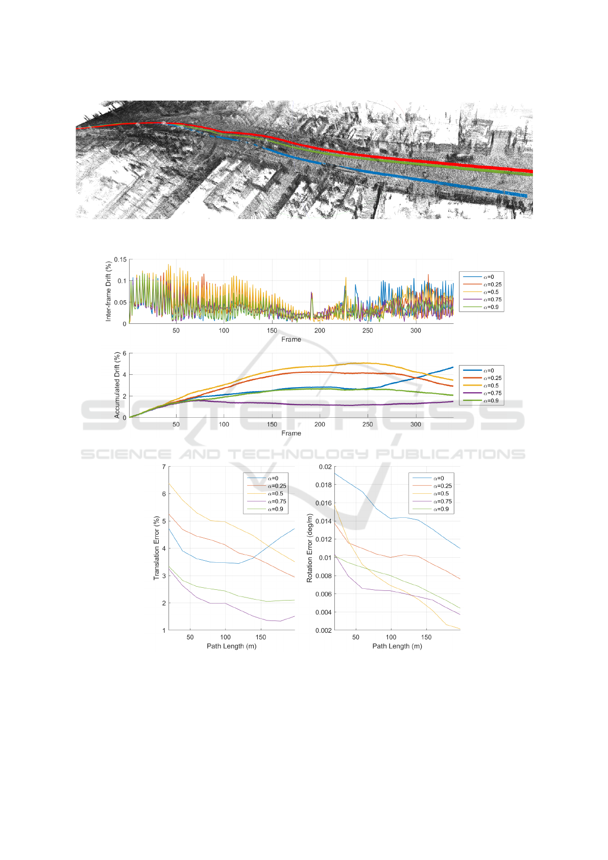
Figure 3: Visualisation of the ego-motion estimated without regularisation α = 0 (blue) and with regularisation α = 0.9
(green). The red line shows the ground truth motion from GPS/IMU data.
Figure 4: Inter-frame drift (top) and accumulated drift (bottom) plots of the tested sequence.
Figure 5: The errors of ego-motion of the translation part (left) and the rotation part (right) with respect to travel distance.
The drifts of the estimated vehicle position are
plotted in Fig. 4. The accumulated error plot shows,
with the regularisation term enabled, that the drift
steadily converged to a lower bound, as observed in
all the four cases where the epipolar constraints took
place during the optimisation phase. We found that,
as more and more pedestrians present in the field of
view, the conventional approach (without regularisa-
tion) starts to deviate from the ground truth. This is
shown in the inter-frame drift plot, from frame 260
Regularised Energy Model for Robust Monocular Ego-motion Estimation
367

thru the end of sequence. A possible reason being
that, those feature points belonging to the moving ob-
jects are falsely triangulated and tracked. Arriving at
the end of the sequence, the regularised energy model
with α set to 0.75 achieved the lowest drift within
1.7% (3 metres), while the conventional re-projection
error minimisation approach presented the worst re-
sult, with a motion drift above 5%.
We also calculated segmented motion errors in
terms of translation and rotation components of the
estimated ego-motion, with respect to various travel
distances. The travel distance is not measured only
from the beginning of the sequence; any segment be-
gins from an arbitrary frame k thru frame k + n where
n > 0 having a length l is taken into account during
the error calculation of interval [l
p
, l
q
) if l
p
≤ l < l
q
.
We divide the length of the sequence into 10 equally
spaced segments for plotting. The results are de-
picted in Fig. 5. It shows that, in the translation com-
ponent, the damping parameter α = 0.75 yields the
best accuracy in all segments, while the conventional
model maintains a moderate accuracy in travel dis-
tances shorter than 100 metres. On the rotation part,
however, it presents the worst accuracy. The best
accuracy, achieved by α = 0.5, which equally relies
on both re-projection and epipolar constraints, is five
times better than the conventional model.
5 CONCLUSIONS
In this paper we reviewed the underlying mathemati-
cal models of the monocular ego-motion estimation
problem and formulated an enhanced minimisation
model to improve the stability and robustness of the
optimisation process.
The experimental findings support a positive ef-
fect of the proposed model on increasing the accu-
racy of the VO procedure. Remarkably, with monoc-
ular vision the presented implementation achieves an
overall motion drift within 2% over 200 metres, which
is comparative to the stereo VO implementations as
listed on the website of the KITTI visual odometry
benchmark in 2016.
REFERENCES
Badino, H., Yamamoto, A., Kanade, T.: Visual odometry by
multi-frame feature integration. Int. ICCV Workshop
Computer Vision Autonomous Driving (2013)
Engels, C., Stewenius, H., Nister, D.: Bundle adjust-
ment rules. In Proc. Photogrammetric Computer Vi-
sion (2006)
Fischler, M.A., Bolles, R.C.: Random sample consensus:
A paradigm for model fitting with applications to im-
age analysis and automated cartography. Comm. of
the ACM, vol. 24, no. 6, pp. 381–395 (1981)
Forster, C., Pizzoli, M., Scaramuzza, D.: SVO: Fast semi-
direct monocular visual odometry. In: Proc. IEEE Int.
Conf. Robotics Automation, pp. 15–22 (2014)
Geiger, A., Lenz, P., Stiller, C., and Urtasun, R.: Vision
meets robotics: The KITTI dataset. Int. J. Robotics
Research, vol. 32, no. 11, pp. 1231–1237 (2013)
Geng, H., Chien, H.-J., Nicolescu, R., Klette, R.: Egomo-
tion estimation and reconstruction with Kalman filters
and GPS integration. In: Proc. Computer Analysis of
Images and Patterns, vol. 9256, pp. 399–410 (2015)
Hartley, R. I., Zisserman, A. : Multiple View Geometry in
Computer Vision, second edition. Cambridge Univer-
sity Press, Cambridge (2004)
Hu, G., Huang, S., Zhao, L., Alempijevic A., Dissanayake,
G.: A robust RGB-D SLAM algorithm. In Proc.:
IEEE/RSJ Int. Conf. on Intelligent Robots and Sys-
tems, pp. 1714–1719 (2012)
Klette, R.: Concise Computer Vision. Springer, London
(2014)
Konolige, K., Agrawal, M.: FrameSLAM: From bundle
adjustment to real-time visual mapping. IEEE Trans.
Robotics, vol. 5, no. 24, pp. 1066–1077 (2008)
Lepetit, V, Moreno-Noguer, F., Fua. P.: EPnP: An accurate
O(n) solution to the PnP problem. Int. J. Computer
Vision, vol. 81, pp. 155–166 (2009)
Levenberg, K.A.: Method for the solution of certain non-
linear problems in least squares. The Quarterly Ap-
plied Math., vol. 2, pp. 164–168 (1944)
Morales, S., Klette, R.: Kalman-filter based spatio-temporal
disparity integration. Pattern Recognition Letters, vol.
34, no. 8, pp. 873–883 (2013)
Sampson, P.D.: Fitting conic sections to ‘very scattered’
data: An iterative refinement of the Bookstein algo-
rithm. Computer Graphics Image Processing, vol. 18,
no. 1, pp. 97–108 (1982)
Scaramuzza, D., Fraundorfer, F.: Visual odometry: Part I
- The first 30 years and fundamentals. IEEE Robotics
Automation Magazine, vol. 18, pp. 80–92 (2011)
Tomasi, C., Kanade, T.: Detection and tracking of point fea-
tures. Carnegie Mellon University Technical Report,
CMU-CS-91-132 (1991)
Vaudrey, T., Badino, H., Gehrig, S.: Integrating disparity
images by incorporating disparity rate. In. Proc. Robot
Vision, LNCS 4931, pp. 29–42 (2008)
Wu, F.C., Zhang, Q., Hu, Z.Y.: Efficient suboptimal solu-
tions to the optimal triangulation. Int. J. Computer Vi-
sion, vol. 91, no. 1, pp. 77–106 (2011)
Zhengyou, Z.: Determining the epipolar geometry and its
uncertainty: A review. Int. J. Computer Vision, vol. 2,
no. 27, pp. 161–198 (1998)
VISAPP 2017 - International Conference on Computer Vision Theory and Applications
368