Noise-resistant Unsupervised Object Segmentation in Multi-view Indoor

Point Clouds

Dmytro Bobkov

, Sili Chen

, Martin Kiechle

, Sebastian Hilsenbeck

and Eckehard Steinbach

Chair of Media Technology, Technical University of Munich, Arcisstr. 21, Munich, Germany

Institute of Deep Learning, Baidu Inc., Xibeiwang East Road, 10, Beijing, China

Chair of Data Processing, Technical University of Munich, Arcisstr. 21, Munich, Germany

NavVis GmbH, Blutenburgstr. 18, Munich, Germany

Keywords:

Object Segmentation, Concavity Criterion, Laser Scanner, Point Cloud, Segmentation Dataset.

Abstract:

3D object segmentation in indoor multi-view point clouds (MVPC) is challenged by a high noise level, varying

point density and registration artifacts. This severely deteriorates the segmentation performance of state-of-

the-art algorithms in concave and highly-curved point set neighborhoods, because concave regions normally

serve as evidence for object boundaries. To address this issue, we derive a novel robust criterion to detect

and remove such regions prior to segmentation so that noise modelling is not required anymore. Thus, a

signiﬁcant number of inter-object connections can be removed and the graph partitioning problem becomes

simpler. After initial segmentation, such regions are labelled using a novel recovery procedure. Our approach

has been experimentally validated within a typical segmentation pipeline on multi-view and single-view point

cloud data. To foster further research, we make the labelled MVPC dataset public (Bobkov et al., 2017).

1 INTRODUCTION

Unsupervised segmentation of 3D indoor scenes into

objects remains a highly challenging topic in com-

puter vision despite many years of research. Seg-

mentation using data from handheld depth sensors,

e.g., Kinect, is a well-studied research topic due to

low price and ﬂexibility (Soni et al., 2015), (Karpathy

et al., 2013) and (Jiang, 2014). Most existing datasets

include only single-view data and focus on small en-

vironments due to the high effort involved in record-

ing building-scale environments using handheld sen-

sors. When recording large indoor environments the

operational costs and time constraints become more

important as the environment has to be free of dy-

namic objects during the time of scanning. Compared

to Kinect-based solutions, laser scanners have a clear

advantage in this context as they provide a larger scan-

ning range (typically more than 30 meters) and wider

angle of view. With these systems, it is possible to

scan an area of ten thousand square meters within a

day, which is practically impossible using any Kinect-

like sensor. A number of mapping platforms equipped

with laser scanners have been developed using either a

wearable backpack (Liu et al., 2010) or a moving trol-

ley (Huitl et al., 2012). The sensors progressively take

measurements and integrate them into a 3D model

using a SLAM system, while the platform is moved

through the indoor space.

As a result of the speciﬁc scanning procedure

required for large indoor environments (e.g., ﬂoors

and buildings), multi-view point cloud (MVPC) data

acquired using a moving platform tend to have the

following drawbacks when compared to single-view

data:

1. Unreliable surface normal information caused by

registration artifacts. These are mostly due to in-

accuracies when registering multiple range scans

into a single 3D map. Such artifacts are most

pronounced in large datasets, because registration

noise tends to accumulate over time (Pomerleau

et al., 2013). This complicates the object segmen-

tation using solely normal information.

2. Varying point density. This is caused by large

scanner setup and strict time constraints, so that it

is, sometimes, simply impossible to scan the ob-

jects from various directions.

The available single-view depth indoor datasets

(N. Silberman and Fergus, 2012), (Lai et al., 2013),

(Xiao et al., 2013) are not representative for building-

scale indoor applications, because of the aforemen-

Bobkov D., Chen S., Kiechle M., Hilsenbeck S. and Steinbach E.

Noise-resistant Unsupervised Object Segmentation in Multi-view Indoor Point Clouds.

DOI: 10.5220/0006100801490156

In Proceedings of the 12th International Joint Conference on Computer Vision, Imaging and Computer Graphics Theory and Applications (VISIGRAPP 2017), pages 149-156

ISBN: 978-989-758-226-4

149

tioned differences to MVPC data. The dataset of

(Song and Xiao, 2014) is not suitable for evalua-

tion of point cloud-based segmentation algorithms be-

cause severe misalignment artifacts are present in the

point cloud data. This is due to the fact that object

labelling has been done in depth images only. The

large dataset of (Armeni et al., 2016) has been cap-

tured using a static laser scanner, which experiences

lower noise level as compared to a moving scanning

platform. This setup is, however, signiﬁcantly limited

for large environments due to small scanning range

and longer capture times. Other available multi-view

datasets are not applicable, because they are either

limited in size and contain only single objects (Mian

et al., 2006) or capture outdoor environments (Boyko

and Funkhouser, 2014), which have different geomet-

ric properties than indoor scenes. To ﬁll this gap be-

tween single-view and multi-view indoor datasets, we

provide an annotated point cloud dataset that reﬂects

these real world constraints. Our dataset spans 6 room

scenes with various objects, such as tables, chairs,

lamps etc. and is made available to the scientiﬁc com-

munity (Bobkov et al., 2017) in order to foster further

research in this area.

Existing approaches for 3D point cloud segmen-

tation are usually tested on single-view datasets.

Hence, they do not consider the important peculiar-

ities of MVPC data and tend to perform poorly on

such datasets. Furthermore, these approaches have

been designed speciﬁcally for depth-based datasets

(Jiang, 2014), (Song and Xiao, 2014), (Deng et al.,

2015), (Fouhey et al., 2014), (Tateno et al., 2015).

Other methods make strong assumptions on scene

planarity (Mattausch et al., 2014). Supervised meth-

ods achieve good segmentation performance (Karpa-

thy et al., 2013), (Soni et al., 2015), but require mas-

sive amount of labelled training examples, which are

unavailable for MVPC datasets. Therefore, this paper

considers unsupervised methods. The performance

of state-of-the-art segmentation methods (Stein et al.,

2014), (van Kaick et al., 2014) on MVPC is not satis-

factory. This is due to the high noise level in highly-

curved concave regions, which normally serve as a

strong evidence for object boundaries (Fouhey et al.,

2014), (Stein et al., 2014). To overcome this limita-

tion, we propose a novel point set-based criterion to

detect such concave noisy regions and temporarily re-

move them prior to scene segmentation. We further

propose a procedure to restore such noisy regions af-

ter initial segmentation.

The contributions of this paper are the following:

• Method to robustly detect high-noise regions.

It helps to overcome limitations of state-of-the-

art object segmentation algorithms that perform

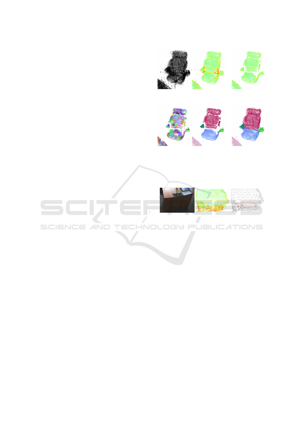
(a) Input data (b) Pre-processed

point cloud

point removal

(d) Supervoxel

clustering

(e) Segmentation (f) Recovery

Figure 1: Processing steps of the analysed segmentation

pipeline. Steps shown in bold are novel contributions of

this paper. Note that curvature values are color coded in (b)

and (c): low value is green and high is red.

(a) RGB image (b) Point cloud (c) Surface graph

Figure 2: Illustration of noisy region inﬂuence (b) on sur-

face graph. In (c) erroneous connections resulting from

noise in a planar region are highlighted. After non-convex

region removal step these noisy points in the planar region

have been removed as well as the erroneous connections.

poorly on MVPC datasets due to the speciﬁc prop-

erties of such data.

• A new MVPC dataset with labelling for objects

and parts. It has been acquired using a laser scan-

ner and contains scenes of ofﬁce environments.

2 METHODOLOGY

To illustrate the improvements achievable with the

proposed concave/convex region criterion, we ﬁrst

consider a typical 3D object segmentation pipeline,

as described in (Stein et al., 2014). One normally

performs pre-processing on the input point cloud

(Fig. 1a) data to remove outliers and other artifacts.

This is typically done in combination with normal and

curvature calculation (Fig. 1b). Afterwards, the su-

pervoxel (surface-patch) adjacency graph is extracted

from the point cloud, e.g., using the approach of (Pa-

VISAPP 2017 - International Conference on Computer Vision Theory and Applications

150

𝑁

= 45

𝑁

= 4

𝑁

= 16

𝑁

−

= 9

𝑁

−

= 24

𝑁

−

= 17

Figure 3: Illustration of high-curvature regions. Left: con-

cave region. Middle: convex region. Right: ambiguous

region. The numbers N

and N

−

indicate the number of

points in positive and negative half-space respectively.

pon et al., 2013), in order to reduce the complex-

ity of the input data (Fig. 1d). Finally, segmenta-

tion is performed on the given graph using a state-

of-the-art graph partitioning method (Fig. 1e). We

propose to augment the segmentation pipeline by the

additional steps of curved non-convex point removal

(Fig. 1c) and recovery according to the proposed cri-

terion (Fig. 1f). We present the details of each of these

steps and discuss the limitations of the state-of-the-art

approaches. We consider point clouds with viewpoint

that is the direction from which the range sensor has

detected this point. For preprocessing (smoothing and

curvature and normal estimation) we use the method

of (Rusu et al., 2008). We have not noticed any signif-

icant improvement when using the estimation method

of (Boulch and Marlet, 2012).

2.1 Classiﬁcation into Convex and

Non-convex Points

Limitation of Supervoxels and Normals. In order

to reduce the computational complexity, we group

points according to the algorithm of (Papon et al.,

2013). It essentially over-segments 3D point cloud

data into patches called supervoxels (Fig. 1d). The

supervoxels are desired not to span boundaries across

objects. Unfortunately, this is not the case for noisy

highly-curved concave regions, which often coincide

with object boundaries. This effect is illustrated in

Fig. 2. Note the false connections (circled in red)

within the wall of the table in the middle of the scene

within a concave high-curvature region. If we would

just remove all high-curvature regions, this would

severely degrade the segmentation performance, be-

cause many of the removed points represent impor-

tant connections within objects that should not be par-

titioned. This effect is not speciﬁc to supervoxels

only, but occurs in any patch-based surface represen-

tation as surface estimation is negatively inﬂuenced

by noise.

Noise-resilient Convexity/Concavity Criterion. We

derive a novel convexity/concavity criterion operating

on point set statistics that is robust to noise in the nor-

mal estimation in order to cope with the aforemen-

tioned limitations. The criterion is deﬁned for the

neighborhood with radius R of a given point ~p. In

particular, for a given point coordinate (p

, p

) and

its normal (n

) (Fig. 3), one can deﬁne a plane

having the same normal as ~n and containing point ~p.

The plane equation is given in Hessian form:

· x + n

· y + n

· z + d = 0, (1)

where d is the distance to the origin and can be com-

puted from (1) by using p

, p

instead of x, y,z.

This tangent plane divides the whole space into two

half-spaces. We compute in which half-space a par-

ticular point is located with (1). By analysing convex

and concave neighborhood regions, we ﬁnd that the

points within R are typically located within the same

half-space as the normal direction ~n for the concave

regions, and for convex ones in the other half-space.

We compare the number of points within each half-

space to determine whether the given point neighbor-

hood R is non-convex and if yes, it will be removed:

m(~p,R) =



non-convex , if N

≥ α

· N

−

convex , if N

< α

· N

−

(2)

where N

is the number of points in the neighborhood

R lying within the same half-space as the normal vec-

tor of the local surface ~n(R), and N

−

is the number

of neighboring points lying within the opposite half-

space and α

is the threshold to detect noisy regions.

We illustrate the choice of the value of α

on the ex-

ample of the regions in Fig. 3. Concave and ambigu-

ous regions need to be removed for the best segmenta-

tion performance. In contrast, convex regions have to

be preserved. For α

= 0.1 the convex region in Fig. 3

is classiﬁed as non-convex and removed. Its removal

leads to over-segmentation of the object. For α

= 1.0

the ambiguous region (that mostly consists of mea-

surement noise) will be classiﬁed as convex and thus

preserved. Experiments on laser scanner data indicate

that with α

= 0.2 such regions will be correctly clas-

siﬁed for the used datasets (see further results in Dis-

cussion). The point neighborhoods satisfying the non-

convex condition in (2) and with curvature θ > θ

will

be temporarily removed (Fig. 1c). From this point

on, we denote concave and ambiguous regions as non-

convex for the sake of simplicity.

2.2 Supervoxel Clustering and Graph

Partitioning

After noisy high-curvature non-convex regions have

been removed, edge weights between neighboring su-

pervoxels can be adequately computed. For this, we

consider supervoxel ~p

= (~x

, ~n

), with centroid ~x

normal vector ~n

and edges to adjacent supervoxels.

Noise-resistant Unsupervised Object Segmentation in Multi-view Indoor Point Clouds

151

We do not want to strictly enforce the condition of

concave object boundaries. Instead, we argue that

concavity is just one indicator for the object bound-

ary and Euclidian distance and surface normals still

serve as evidence for object boundaries in case of non-

concave regions. Therefore, we calculate the graph

edge weight between neighboring supervoxels as fol-

lows:



a · D

, if convex edge

D , if concave edge,

(3)

where D is the deﬁnition for edge weight described in

(Papon et al., 2013), but implemented differently by

the authors in Point Cloud Library:

D =

|~x

−~x

seed

· w

+ (1 − | cos(~n

,~n

)|) · w

, (4)

where |~x

−~x

| is the Euclidean distance between two

nodes (centroids of supervoxel patches), R

seed

is the

seed radius,~n

and~n

are normals of two supervoxels

and w

are spatial and normal weights, respec-

tively. Note that we omit the color difference term

compared to original formulation as it does not nec-

essarily improve segmentation results, also observed

in (Karpathy et al., 2013). The parameter a denotes

the weight for considering the importance of concav-

ity when partitioning objects. A lower value for a in-

creases the weight of the concavity criterion in the

segmentation process. Based on experimental results

and to be able to segment various objects, we strike a

trade-off by using a = 0.25 for all experiments. From

(3), it is clear that in case of similar weights con-

cave edges will be preferred as object boundaries in

most cases. Nonetheless, in case a convex edge con-

nects two remotely located regions with drastically

different surface, the spatial and normal distance can

serve as evidence for object partitioning. Similarly

to (Stein et al., 2014), we set R

seed

voxel

= 4 for all

used datasets, where R

voxel

is the voxel radius. In our

experiments, we set w

= 0.2 and w

= 0.5 for all

datasets, as we have observed that normal information

is more characteristic when describing the surface ge-

ometry compared to the Euclidian distance.

When partitioning the extracted graph of scenes

with complex geometry, we observed that sim-

ple region-growing algorithms do not perform well.

Therefore, we instead use adaptive statistics-based

graph-based segmentation algorithm of (Felzen-

szwalb and Huttenlocher, 2004) (Fig. 1e). Other

graph partitioning algorithms, such as spectral clus-

tering and normalized mincut do not achieve such a

good trade-off between accuracy and speed.

2.3 Recovery of Previously Removed

Noisy Non-convex Points

It is necessary to recover the removed non-convex

high-curvature points and assign them to correct la-

bels. While recovering such points, the most similar

labelled points in the vicinity need to be determined.

The local surface geometry is important for this pur-

pose. For this reason, we use the graph edge weight

deﬁned in (4) as our similarity metric. We have ob-

served that simple region growing algorithms based

on seeds (i.e. known labels) are sensitive to outliers,

which often occur at such highly-curved regions. To

overcome this problem, we constrain the number of

propagated labels per iteration. Furthermore, we start

with connections having lower weights as these ex-

hibit higher similarity and compute this metric in the

vicinity R

voxel

of the given point. Within one iter-

ation, we limit the number of points to recover to

a certain percentage P

of the number of currently

unlabelled points that have labelled neighbors (P

80%). We have experimentally found that K = 20

such iterations are sufﬁcient to recover non-convex

points (observe an example of the restored labels in

Fig. 1f). The pseudocode for the algorithm is given

in Algorithm 1. Here LabelledRadiusPoints(P,R) re-

turns labelled neighboring points around P within the

search radius R. LabelO f (P) returns the point label.

Note that W denotes a triplet with point, distance and

weight.

Algorithm 1: Label Removed Non-convex Points.

Q ← labelled points

U ← unlabelled points

for k = 0 to K − 1 do

W ← {}

for all P

∈ U do

M ← LabelledRadiusPoints(P

Voxel

)

if M 6=

0 then

jmin ← argmin

∀M

∈M

D(P

)

min

← D(P

jmin

) (4)

min

← LabelO f (M

jmin

)

W ← W ∪ {M

jmin

min

}

if k 6= K − 1 then

Sort W with ascending order of D

Preserve

← Rnd(Length(W ) · P

)

for i = 0 to N

Preserve

− 1 do

Q ← Q ∪W

3 EXPERIMENTAL EVALUATION

In this section, we present quantitative results on

manually labelled laser scanner-based indoor point

VISAPP 2017 - International Conference on Computer Vision Theory and Applications

152

cloud data. We further provide experimental results

for Kinect data. We benchmark our results against

the state-of-the-art geometry-based unsupervised seg-

mentation algorithms of (Stein et al., 2014) (Locally

Convex Connected Patches - LCCP) and (van Kaick

et al., 2014). For this, we use the publicly accessible

algorithm implementations provided by the authors.

3.1 Laser Scanner Dataset and

Evaluation Metric

For rigorous evaluation of various segmentation ap-

proaches and due to the lack of publicly available

multi-view point cloud datasets, we manually label

6 indoor scenes by specifying object parts and their

relationship to each other. The point cloud data has

been acquired using a mobile mapping platform with

3 Hokuyo UTM-30LX laser scanners. While the anal-

ysis can be done on the data from any range sensor,

we chose laser scanners as they offer a fast acquisi-

tion procedure in large indoor environments. As the

platform is moved through the environment, its laser

scanners perform range measurements in one hori-

zontal and two intersecting vertical planes, thus in-

crementally building a 3D map. The average scan-

ning time per room constitutes several minutes. The

captured scenes represent typical ofﬁce environments

with various objects. The total number of objects is

156, which contain 452 semantic object parts (e.g.

chair back, leg, arm etc., see Fig. 4).

When labelling, some may regard a chair as a

whole object, while others may regard it as a col-

lection of parts, such as chair back, chair leg etc. It

is unclear which of this labelling is correct. There-

fore, we derive labelling on several object levels, e.g.

ﬁne and coarse ground truth (GT). Fine GT includes

object parts, while coarse GT capture objects them-

selves. Finally, the proper GT given the segmenta-

tion result will be generated based on the predicted

label as well as coarse and ﬁne GT data. Prior to la-

belling, we employ plane segmentation to remove ar-

chitectural parts of buildings, such as walls and ﬂoor.

Furthermore, due to the rather coarse resolution of the

point clouds, we do not separately label small objects

that are not distinguishable from noise, e.g., the pen

lying on the table. As an evaluation metric, we pro-

pose an extension to under-segmentation (UE) ME

and over-segmentation error (OE) ME

that was ﬁrst

mentioned in (Richtsfeld et al., 2012). Compared to

the original version, we evaluate with respect to an

object and its parts so that most appropriate GT is

considered (see (Bobkov et al., 2017) for details).

Table 1: Comparison of the segmentation methods on the

laser scanner data. Used error metric is multi-scale over-

and under-segmentation, where smaller is better. Top value

is ME

and bottom value is ME

. Bold entries indicate

best performance per scene. Average processing time of our

approach is less than 10s per scene.

Scene Our LCCP Our+LCCP van Kaick

15.3% 35.8% 23.8% 37.1%

5.6% 12.2% 6.5% 16.3%

6.2% 30.4% 20.2% 25.6%

0.6% 9.0% 6.1% 23.6%

10.9% 20.5% 17.3% 17.7%

8.9% 9.7% 6.1% 78.7%

8.8% 18.8% 11.0% 32.9%

17.5% 143.7% 88.3% 647.8%

6.6% 29.6% 22.3% 27.8%

8.7% 23.2% 4.3% 80.8%

15.1% 21.2% 17.7% 37.6%

12.5% 36.9% 28.8% 104.4%

Mean

11.4% 26.0% 18.8% 29.8%

8.9% 39.1% 23.3% 158.6%

3.2 Experimental Results

Laser Scanner SLAM Dataset. We ﬁrst present re-

sults scene-wise in Table 1. Here we include results

for the two aforementioned algorithms (LCCP and

van Kaick), as well as a combination of our criterion

(non-convex region removal and recovery) with the

LCCP segmentation algorithm (”Our+LCCP”). For

all laser scanner-based room datasets we used the

same parameters for our method, in particular R

seed

12cm, C = 3, θ

= 0.03, k = 3, thus no parameter tun-

ing for a particular scene has been performed. For

LCCP we used same R

voxel

and R

seed

, while other pa-

rameters are described in (Stein et al., 2014). From

the results in Table 1 one can observe that the pro-

posed algorithm signiﬁcantly outperforms LCCP as

well as the approach of (van Kaick et al., 2014) for

both multi-scale UE and OE. The three scenes along

GT data and segmentation results of the analyzed al-

gorithms are provided in Fig. 4. Observe in the right

column of Fig. 4 the case when LCCP segmentation

deteriorates due to noisy normals. One can see that

the high UE of LCCP stems from the fact that it has

merged the chair in the top part of the scene with the

table. The method of (van Kaick et al., 2014) also

shows limited performance on partitioning the table

from the adjacent chairs. In contrast, the proposed

method has produced better results by separating the

chairs from the table. Limited LCCP performance

is mostly due to noisy normals and low-density re-

gions in the neighborhood of chairs. The method of

Van Kaick et al. is limited on such scenes as it can-

not handle sparsity in the data. On the other hand,

our method is more robust with respect to such re-

Noise-resistant Unsupervised Object Segmentation in Multi-view Indoor Point Clouds

153

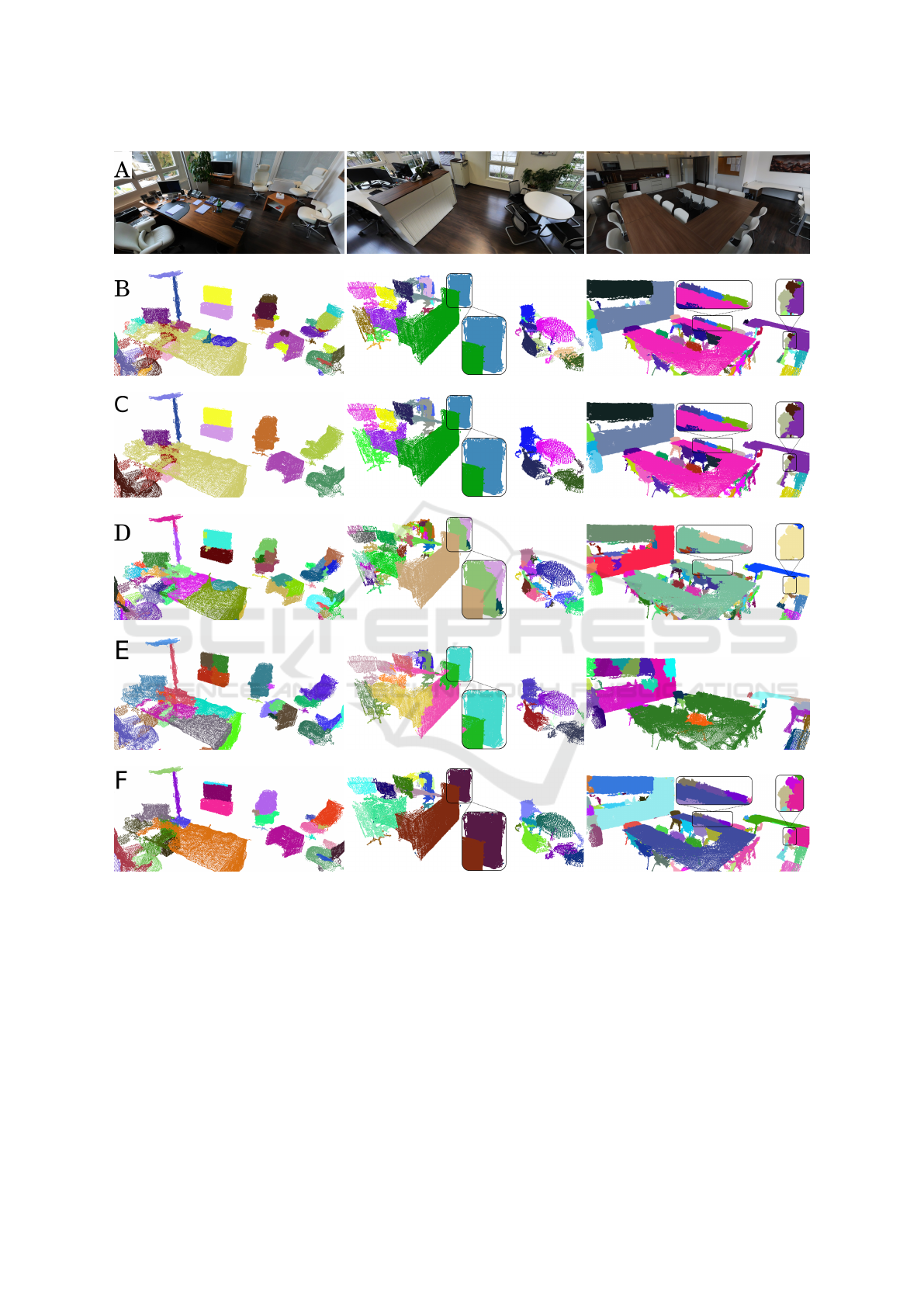
Figure 4: Example results for manually labelled scenes 1, 3 and 4 (left, middle and right column respectively). Here row A

is given for illustration, but not used by any of the algorithms. B is the ﬁne GT. C illustrates coarse GT. D represents LCCP

segmentation results. E shows segmentation results of the approach of (van Kaick et al., 2014). F corresponds to segmentation

results of the proposed method.

gions. Furthermore, observe that LCCP as well as our

method have over-segmented the left part of the scene

containing kitchen cupboards and objects on the table.

And ﬁnally, in the right part of the scene, both algo-

rithms are unable to correctly segment the corner ta-

ble, thus increasing OE. For scene 3 (middle column

of Fig. 4), LCCP over-segments the objects behind

the cupboard in the upper part of the scene, whereas

our method correctly segments such parts, and thus

has a lower OE. The method of (van Kaick et al.,

2014) shows high UE on this scene. Also note that our

convex/concave criterion combined with LCCP algo-

rithm (”Our+LCCP”) gives clear improvement.

NYU Dataset. We further evaluate the algorithms on

the NYUv2 Kinect dataset (N. Silberman and Fergus,

2012). It contains 1449 scenes with realistic cluttered

conditions, captured from a single viewpoint. Quanti-

tative evaluation on 654 test scenes is provided in Ta-

VISAPP 2017 - International Conference on Computer Vision Theory and Applications

154

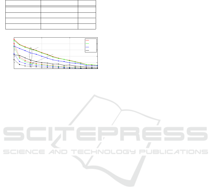
Table 2: Performance of segmentation methods on the NYU

dataset using weighted overlap (WO) (bigger is better).

Method Learned features WO

Proposed No learning 58.0%

LCCP No learning 57.6%

Silberman et al. Depth 53.7%

Gupta et al. Depth+RGB 62.0%

0 0.05 0.1 0.15

Curvature threshold θ

0.2

0.4

0.6

0.8

Relative number of

removed edges

=0.1

=0.2

=0.5

=1.0

Inter-object connections

Intra-object connections

Figure 5: Gain achieved by removing non-convex noisy

regions vs. curvature threshold θ

- signiﬁcant number of

inter-object connections are removed (solid). Note the low

number of removed intra-object connections (dashed).

ble 2. We used θ

= 0.02, C = 3, k = 5, R

seed

= 16cm

for all scenes. For comparison we also provide the

performance of LCCP and training-based methods of

(N. Silberman and Fergus, 2012) and (Gupta et al.,

2013). Observe that our method achieves reasonable

performance in spite of being learning-free, as com-

pared to (Gupta et al., 2013).

Parameter Sensitivity. For illustration of the cur-

vature threshold θ

we show the number of inter-

object vs. intra-object edges that are removed in the

laser scanner dataset in Fig. 5. One can see that by

choosing its value in the range 0.02 to 0.03 a signiﬁ-

cant number of inter-object connections are removed

(e.g. 68.31%), whereas most of the intra-object con-

nections are preserved (e.g. 77.21%). This allows

us to signiﬁcantly simplify the segmentation problem

while achieving even better performance. Please note

that we also varied α

, which conﬁrms the choice of

= 0.2 for this dataset. Due to marginal improve-

ment, we ﬁx parameter k = 3 for all scenes in the laser

scanner dataset. We want to point that the parameter

k offers the trade-off between UE and OE, in particu-

lar higher k would result in lower OE and higher UE.

Should one thrive for low UE, the parameter k has

to be reduced. The parameter for graph partitioning

C should be chosen jointly with seed resolution R

seed

depending on the desired size of the smallest segment.

Finally, R

seed

should be greater than the average point

cloud resolution, as indicated in (Papon et al., 2013).

Limitations. Removing high-curvature non-convex

regions can sometimes result in the situation that

some regions become too sparse, therefore no connec-

tions within the object remain. This, apparently, will

lead to erroneous over-segmentation of the object. We

further acknowledge the simplicity of the used crite-

rion of a concave edge, which can fail in some cases

(TV set in scene 1 in Fig. 4).

4 CONCLUSION

This paper presents a novel approach for segmen-

tation of multi-view indoor point clouds. To ad-

dress particular properties of these datasets, such as

non-uniform density and high level of noise, we de-

rived a novel noise-resilient criterion for the detection

of noisy non-convex regions. This step makes the

graph partitioning (and thus segmentation) problem

simpler and reduces the number of erroneous con-

nections due to noise. By combining the proposed

point removal step with state-of-the-art segmentation

algorithms, one can signiﬁcantly improve their per-

formance. In spite of being designed for MVPC data,

the algorithm achieves state-of-the-art performance

on single-view point cloud data. We further introduce

a new laser scanner dataset to illustrate experimen-

tally that there is a discrepancy between single-view

and multi-view point clouds in terms of noise level,

especially at high-curvature regions. The proposed

dataset spans 6 rooms within an ofﬁce environment

and contains 452 object parts. It is especially valu-

able to the scientiﬁc community as the moving laser

scanner-based approaches are particularly suitable for

the mapping and 3D reconstruction of large indoor en-

vironments.

REFERENCES

Armeni, I., Sener, O., Zamir, A. R., Jiang, H., Brilakis,

I., Fischer, M., and Savarese, S. (2016). 3d seman-

tic parsing of large-scale indoor spaces. In Proceed-

ings of the IEEE International Conference on Com-

puter Vision and Pattern Recognition.

Bobkov, D., Chen, S., Kiechle, M., Hilsenbeck,

S., and Steinbach, E. (2017). Supplementary

material for paper: Noise-resistant unsupervised

object segmentation in multi-view indoor point

clouds. https://github.com/DBobkov/segmentation.

Accessed: 2016-11-29.

Boulch, A. and Marlet, R. (2012). Fast and robust normal

estimation for point clouds with sharp features. Com-

puter Graphics Forum, 31(5):1765–1774.

Boyko, A. and Funkhouser, T. (2014). Cheaper by the

dozen: Group annotation of 3D data. In UIST.

Deng, Z., Todorovic, S., and Jan Latecki, L. (2015). Se-

mantic segmentation of rgbd images with mutex con-

straints. In The IEEE International Conference on

Computer Vision (ICCV).

Noise-resistant Unsupervised Object Segmentation in Multi-view Indoor Point Clouds

155

Felzenszwalb, P. F. and Huttenlocher, D. P. (2004). Efﬁ-

cient graph-based image segmentation. International

Journal on Computer Vision, 59(2):167–181.

Fouhey, D., Gupta, A., and Hebert, M. (2014). Unfold-

ing an indoor origami world. In Fleet, D., Pajdla, T.,

Schiele, B., and Tuytelaars, T., editors, Computer Vi-

sion ECCV 2014, volume 8694 of Lecture Notes in

Computer Science, pages 687–702. Springer Interna-

tional Publishing.

Gupta, S., Arbelez, P., and Malik, J. (2013). Perceptual or-

ganization and recognition of indoor scenes from rgb-

d images. In Computer Vision and Pattern Recogni-

tion (CVPR), 2013 IEEE Conference on, pages 564–

571.

Huitl, R., Schroth, G., Hilsenbeck, S., Schweiger, F., and

Steinbach, E. (2012). TUMindoor: an extensive image

and point cloud dataset for visual indoor localization

and mapping. In IEEE International Conference on

Image Processing (ICIP 2012), Orlando, FL, USA.

Jiang, H. (2014). Finding approximate convex shapes in

rgbd images. In Computer Vision ECCV 2014, vol-

ume 8691 of Lecture Notes in Computer Science,

pages 582–596. Springer International Publishing.

Karpathy, A., Miller, S., and Fei-Fei, L. (2013). Ob-

ject discovery in 3D scenes via shape analysis. In

Robotics and Automation (ICRA), 2013 IEEE Inter-

national Conference on, pages 2088–2095.

Lai, K., Bo, L., Ren, X., and Fox, D. (2013). Rgb-d object

recognition: Features, algorithms, and a large scale

benchmark. In Consumer Depth Cameras for Com-

puter Vision, pages 167–192. Springer.

Liu, T., Carlberg, M., Chen, G., Chen, J., Kua, J., and Za-

khor, A. (2010). Indoor localization and visualization

using a human-operated backpack system. In Indoor

Positioning and Indoor Navigation (IPIN), 2010 In-

ternational Conference on, pages 1–10.

Mattausch, O., Panozzo, D., Mura, C., Sorkine-Hornung,

O., and Pajarola, R. (2014). Object detection and

classiﬁcation from large-scale cluttered indoor scans.

Computer Graphics Forum, 33(2):11–21.

Mian, A., Bennamoun, M., and Owens, R. (2006). Three-

dimensional model-based object recognition and seg-

mentation in cluttered scenes. Pattern Analysis

and Machine Intelligence, IEEE Transactions on,

28(10):1584–1601.

N. Silberman, D. Hoiem, P. K. and Fergus, R. (2012). In-

door segmentation and support inference from RGBD

images. In ECCV.

Papon, J., Abramov, A., Schoeler, M., and Worgotter, F.

(2013). Voxel cloud connectivity segmentation - su-

pervoxels for point clouds. In Computer Vision and

Pattern Recognition (CVPR), 2013 IEEE Conference

on, pages 2027–2034.

Pomerleau, F., Colas, F., Siegwart, R., and Magnenat, S.

(2013). Comparing icp variants on real-world data

sets. Autonomous Robots, 34(3):133–148.

Richtsfeld, A., Morwald, T., Prankl, J., Zillich, M., and

Vincze, M. (2012). Segmentation of unknown ob-

jects in indoor environments. In Intelligent Robots and

Systems (IROS), 2012 IEEE/RSJ International Con-

ference on, pages 4791–4796.

Rusu, R. B., Marton, Z. C., Blodow, N., Dolha, M., and

Beetz, M. (2008). Towards 3D point cloud based ob-

ject maps for household environments. robotics and

autonomous systems.

Song, S. and Xiao, J. (2014). Sliding shapes for 3d object

detection in depth images. In Computer Vision–ECCV

2014, pages 634–651. Springer International Publish-

ing.

Soni, N., Namboodiri, A. M., Jawahar, C., and Rama-

lingam, S. (2015). Semantic classiﬁcation of bound-

aries of an RGBD image. In Proceedings of the

British Machine Vision Conference (BMVC 2015),

pages 114.1–114.12. BMVA Press.

Stein, S., Schoeler, M., Papon, J., and Worgotter, F. (2014).

Object partitioning using local convexity. In Com-

puter Vision and Pattern Recognition (CVPR), 2014

IEEE Conference on, pages 304–311.

Tateno, K., Tombari, F., and Navab, N. (2015). Real-

time and scalable incremental segmentation on dense

slam. In Intelligent Robots and Systems (IROS), 2015

IEEE/RSJ International Conference on, pages 4465–

4472. IEEE.

van Kaick, O., Fish, N., Kleiman, Y., Asaﬁ, S., and Cohen-

Or, D. (2014). Shape segmentation by approximate

convexity analysis. ACM Transactions on Graphics.

Xiao, J., Owens, A., and Torralba, A. (2013). Sun3d: A

database of big spaces reconstructed using sfm and

object labels. In Computer Vision (ICCV), 2013 IEEE

International Conference on, pages 1625–1632.

VISAPP 2017 - International Conference on Computer Vision Theory and Applications

156