Parallelized Flight Path Prediction using a Graphics Processing Unit

Maximilian G

otzinger

, Martin Pongratz

, Amir M. Rahmani

2,3

and Axel Jantsch

Department of Information Technology, University of Turku, Turku, Finland

Institute of Computer Technology, TU Wien, Vienna, Austria

Department of Computer Science, University of California, Irvine, U.S.A.

Keywords:

CUDA, GPU, Canny, RANSAC, Image Processing, Parallel Algorithm, Flight Path Prediction, Based on

Memorized Trajectories.

Abstract:

Summarized under the term Transport-by-Throwing, robotic arms throwing objects to each other are a vision-

ary system intended to complement the conventional, static conveyor belt. Despite much research and many

novel approaches, no fully satisfactory solution to catch a ball with a robotic arm has been developed so far. A

new approach based on memorized trajectories is currently being researched. This paper presents an algorithm

for real-time image processing and ﬂight prediction. Object detection and ﬂight path prediction can be done

fast enough for visual input data with a frame rate of 130 FPS (frames per second). Our experiments show

that the average execution time for all necessary calculations on an NVidia GTX 560 TI platform is less than

7.7ms. The maximum times of up to 11.7ms require a small buffer for frame rates over 85 FPS. The results

demonstrate that the use of a GPU (Graphics Processing Unit) considerably accelerates the entire procedure

and can lead to execution rates of 3.5× to 7.2× faster than on a CPU. Prediction, which was the main focus of

this research, is accelerated by a factor of 9.5 by executing the devised parallel algorithm on a GPU. Based on

these results, further research could be carried out to examine the prediction system’s reliability and limitations

(compare (Pongratz, 2016)).

1 INTRODUCTION

Customer needs and requirements are becoming in-

creasingly personalized in almost all product ﬁelds.

Manufacturers have to produce a large number of

products that are similar, but not completely identical.

As not every personalized product has to pass through

the same production stages, the currently used static

conveyor belt no longer matches the application pro-

ﬁle; more ﬂexible types of product lines are needed.

Transport-by-Throwing (Pongratz et al., 2012) de-

scribes an alternative solution whereby robot arms

pass on their payload: one throws it, and another

one catches it. Just as with communication networks

with hop-by-hop routing, passing is repeated until the

transport good reaches its ﬁnal destination in the pro-

duction process. Despite many novel approaches, a

fully satisfactory solution to catch an object has not

yet been developed. In the last 25 years, many other

studies (B

auml et al., 2011; Hong et al., 1995) have

been concerned with the topic of catching a thrown

ball, but the best results achieved a success rate of

about 80% or less. All of these studies has one fact

in common; the predictions are based on a model of

the involved physical laws. Pongratz et al. propose

a strategy based on memorized trajectories (Pongratz

et al., 2010; Pongratz, 2016).

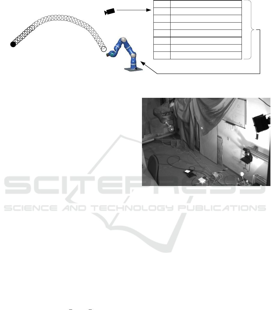
The hypothesis is that humans learn object-

catching based on experience, for example, the way

a child learns to catch a ball. It does not contem-

plate about physics when trying to catch. A child only

learns from its experiences: after numerous failed at-

tempts, it is able to catch an object in the right way

based on memorized previous experience. By anal-

ogy, in the approach proposed by Pongratz et al. the

ball’s ﬂight is captured and compared with a set of

stored reference (Figure 1) throws to enable predic-

tion of the trajectory and the location where the ob-

ject can be caught (Pongratz et al., 2012). Although

the execution time of the prediction is as important

as its accuracy, its real-time constraints have not been

examined until now (Pongratz et al., 2010). If the esti-

mation algorithm takes up too much of the processor’s

capacity, the computation time will interfere with the

camera’s sample rates (Hong et al., 1995). Image pro-

cessing, as well as the comparison of the determined

386

GÃ˝utzinger M., Pongratz M., Rahmani A. and Jantsch A.

Parallelized Flight Path Prediction using a Graphics Processing Unit.

DOI: 10.5220/0006105903860393

In Proceedings of the 12th International Joint Conference on Computer Vision, Imaging and Computer Graphics Theory and Applications (VISIGRAPP 2017), pages 386-393

ISBN: 978-989-758-227-1

pos

traj

pos

...

pos

...

pos

...

pos

...

pos

...

pos

...

pos

...

pos

...

pos

Figure 1: The Transport-by-Throwing approach deals with a robot arm that catches thrown objects with the help of a prediction

based on stored trajectories.

data with all the numerous database entries, require a

huge number of calculation steps. Managing the mas-

sive amount of computation in a short period leads

to the necessity of employing high-performance hard-

ware/accelerators. An FPGA (Field Programmable

Gate Array) based implementation can accelerate the

procedure (Pongratz, 2009), but this would result in

higher development costs. A GPU (Graphics Pro-

cessing Unit) can speed up the software wholly or

partially by parallelizing the operations (Fung et al.,

2005).

In this paper, we deal with such real-time con-

straints and deploy GPUs for performing both object

detection as well as ﬂight path prediction. The here

stated results shall enable examination of the system’s

accuracy in future works.

The rest of the paper is organized as follows. The

concepts and the setup are described in Section 2.

Section 3 shows our implementation of the RANSAC

algorithm and the ﬂight path prediction. In Section 4,

we present and discuss the results from our experi-

ments. Finally, Section 5 concludes the paper.

2 SETUP AND CONCEPT

The ability to catch a thrown object requires knowl-

edge about the trajectory and other attributes of the

motion of the object (Barteit et al., 2009), which we

gather with cameras. The thrown object is a tennis

ball with a velocity from 4.6

to 5.4

. The light sys-

tem consists of multiple ﬂoodlights and results in a

sufﬁcient illumination of the whole scene. Changing

light intensity is compensated by a light proﬁle for

the algorithm which inﬂuences the thresholds of the

detection algorithms. The distance of the ball to each

camera is in the range of 0.6m to 3.2m. Figures 2

and 3 show the experimental setup that is brieﬂy ex-

plained here in this section.

Figure 2: The Throwing-and-Catching test environment

consists in a robot arm, multiple LED ﬂoodlights, two par-

allel aligned cameras, and a throwing device that accelerates

a tennis ball to overcome the distance of about 2.5m.

2.1 Capturing the Scene

Obtaining a 3D view of a scene using only one cam-

era potentially results in low-level accuracy and ro-

bustness (B

auml et al., 2011). Therefore, we opted

to use two cameras (IDS uEye UI-3370CP) working

synchronously and manually aligned in parallel with

a baseline distance of approximately 0.92m. These

two cameras support a resolution of 2048-by-2048

pixels at a frame rate of 75FPS (frames per second)

and 2048-by-800 pixels at 110FPS. To predict the

ﬂight path in time while still having the advantages of

this high resolution, a cropping system based on Bi-

nary Large Objects (BLOBs) detection was used that

provides output images with only 300-by-300 pixels

where the ball is roughly in the center.

The following hardware was used for image pro-

cessing and ﬂight path prediction: a computer with

an i7-4770S CPU clocked at 3.10GHz, 8GB main

memory clocked at 667MHz and an NVidia GeForce

GTX 560 Ti graphics card (NVidia, 2015) with 384

cores (with compute capability 2.1). This GPU fam-

Parallelized Flight Path Prediction using a Graphics Processing Unit

387

Figure 3: This coil-based throwing device accelerates a ten-

nis ball to overcome the distance of about 2.5m.

ily was used as it is a rather standard representative

of GPUs in general. Other - more up to date - GPUs

would change the speciﬁc ﬁgures but not the general

trend and conclusion. Besides, Intel claims that its

integrated GPUs are starting to get equal with dis-

crete graphics cards

. To have also some results for

Catching-and-Throwing devices based on embedded

system, we chose this - weak - graphics processor.

2.2 Detecting the Flying Object

After a coil-based throwing device (Figure 3) ac-

celerated the tennis ball, it appears on both camera

images. Various methods for detecting circles ex-

ist (D’Orazio et al., 2002) but two of them are well-

known, distinguished by their accuracy, and often

used for object detection: the Hough Transformation

and the RANSAC algorithm. Both procedures per-

form efﬁciently when images are not noisy, but the

Hough Transformation was highlighted as being more

accurate when detecting objects in the presence of

noise (Jacobs et al., 2013). On the other hand, the

duration of this algorithm depends on the number of

pixels in the edge image (Wu et al., 2012). One cir-

cle is drawn in the Hough Space for each possible

radius around each edge pixel. Therefore, the more

pixels present, the more time is needed. In compar-

ison, the time required by the RANSAC algorithm

only depends on the number of iterations. The algo-

rithm chooses randomly three points to span a pos-

sible circle. In other words, only one circle is drawn

per iteration; not for every possible radius as it was for

the Hough Transformation. Since the number of iter-

ations needed is much less than the number of edge

pixel multiplied by possible radii, the RANSAC algo-

rithm performs typically faster.

Both algorithms require an edge image for detect-

ing objects in an accurate way. We use the Canny

http://www.extremetech.com/extreme/221322-intel-

claims-its-integrated-gpus-now-equal-to-discrete-cards

Edge Detector algorithm since it achieves good re-

sults and is commonly used (Luo et al., 2008). Its

implementation is carried out in four steps: Gaus-

sian ﬁltering, Sobel ﬁltering, non-maximum suppres-

sion, and hysteresis thresholding (Ogawa et al., 2010).

The ﬁrst three procedures are linearly separated in x-

and y-direction so that they run efﬁciently on parallel

hardware (Luo et al., 2008). In contrast to these steps,

the hysteresis thresholding is an iterative algorithm.

Therefore, this step is not parallelizable and limits the

performance of edge detection.

To improve the quality of the edge images, the im-

ages’ backgrounds can be subtracted as an additional

step. Changing lighting conditions may lead to a non-

perfect background subtraction, but the edge images

and consequently the detection is still more accurate.

2.3 Flight Path Prediction

After the ball’s center point has been detected in both

images, the triangulation step converts these two po-

sitions to one 3D position. Due to the imperfect align-

ment of the stereo vision system, the distortion of the

cameras, and other effects, the vision system has been

calibrated with the help of a Matlab toolbox

. The

result of the calibration process are the intrinsic pa-

rameters of the individual cameras (e.g., focal length,

distortion coefﬁcients) and the extrinsic parameters of

the stereo system (baseline and orientation).

Since every pair of frames offer a new position

of the thrown ball, its movement in space and time is

known. From that moment, we can start the prediction

of the ball’s further ﬂight path. Figure 4 shows two

different approaches for estimating a ﬂight path based

on this technique: either comparing the ball’s posi-

tions with their counterparts in the database directly

or comparing the rates of change from one position to

the next. Because of the high similarity of both ver-

sions, we introduce only the former. To ﬁnd the most

similar trajectory, the Euclidean distances between

each position of the actual ﬂight and its counterpart

in the database are calculated. Afterwards all these

distances are added up to a total distance, which gives

information on how well the actual ﬂight matches a

database trajectory. The database trajectory that leads

to the smallest sum of distances is the most simi-

lar trajectory and is, therefore, selected to predict the

ﬂight path of the thrown tennis ball. One challenge of

this algorithm lies in the enormous number of possi-

bilities to ﬁt the actual ﬂight in a reference trajectory.

Four examples of possible ﬂight paths compared with

one and the same trajectory of the database are shown

Available at: http://www.vision.caltech.edu/bouguetj/

calib doc/

VISAPP 2017 - International Conference on Computer Vision Theory and Applications

388

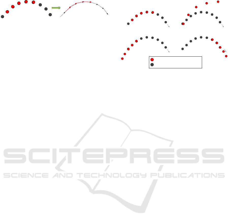
Figure 4: The two prediction approaches: comparing di-

rectly the balls positions, or comparing its rates of change

from one position to the next.

in Figure 5. While the ﬁrst example represents a fairly

good match, the second example shows a lack of con-

gruence between the two ﬂight paths. However, the

reason might be that the actual ﬂight’s positions are

not present in the database trajectory which still ﬁts

best (examples 3 and 4 of Figure 5).

2.4 Software Development Environment

Two options for programming a GPU exist: CUDA

(Compute Uniﬁed Device Architecture) (NVidia,

2014), which was developed by NVidia in 2006 and

OpenCL (Open Computer Language) by the Khronos

Group (Khronos, 2015). We selected CUDA as de-

velopment environment because of its better perfor-

mance (Karimi et al., 2010), and a more comprehen-

sive documentation.

3 IMPLEMENTING

PARALLELIZED FLIGHT PATH

PREDICTION

Based on the edge image object detection is per-

formed. Because the background subtraction is sim-

ple to implement and parallelized algorithms for the

Canny Edge Detector (Luo et al., 2008), the Hough

Circle Transformation (Askari et al., 2013; Chen

et al., 2011), and the RANSAC algorithm (Wang

et al., 2011) have been reported before, we do not de-

scribe their implementation in detail. Instead, we fo-

cus on the ﬂight path prediction. We show the perfor-

mance differences of all algorithms in Section 4; also

the comparison of the straight-forward and inverse-

checking version of the Hough Circle Transforma-

tion (Askari et al., 2013; Chen et al., 2011).

To enable database access as fast as possible, an

initializing function loads all reference trajectories

and stores the data in the GPU’s memory in a 3D array

as a ﬁrst step (similar to (Gowanlock et al., 2015)).

These three dimensions are needed for the different

trajectories, the trajectories’ various positions, and the

positions’ various coordinates. The size of the GPU’s

memory limits the number of reference throws, but

as has been shown (Pongratz, 2016), small databases

also lead to acceptable catching results.

example 1 example 2

example 3 example 4

positions of the actual flightpaths

positions of a database trajectory

Figure 5: Four examples comparing actual ﬂight paths with

the same database trajectory.

The challenge of the ﬂight path prediction algo-

rithm lies in the enormous number of possibilities to

ﬁt the actual ﬂight in all reference trajectories. On the

one hand, many reference trajectories exist that have

to be compared with the actual ﬂight, and on the con-

trary, many different possibilities exist on how to ﬁt

the actual ﬂight in a reference trajectory (Figure 5).

Next we describe our algorithm which makes use of

the parallel architecture of a GPU.

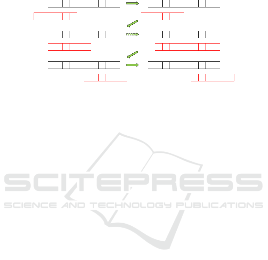
To examine every possibility, the actual ﬂight’s

positions are shifted over the various trajectories of

the database. Additionally, the possibility must be

included that not all the actual positions are aligned

with their counterpart in the database trajectory. Fig-

ure 6 shows such a shift of one actual ﬂight over one

database trajectory. However, since the focus is on

a parallelized algorithm, the term “shift” is not com-

pletely correct. Each database trajectory is examined

in a separate block, and each possible alignment of

the actual ﬂight with a database trajectory is exam-

ined in a separate thread. Therefore, for each of the

database’s trajectories one block exists, and for each

possibility to ﬁt the actual ﬂight, a thread is needed

and created. Since all blocks have to have the same

number of threads, the number of required threads de-

pends on the longest database trajectory. Separating

the examinations of the various alignments in differ-

ent threads is equal to parallelizing the act of shifting

the actual ﬂight over a database trajectory.

To speed up the whole procedure, all positions of

the actual ﬂight and database trajectories are moved

from the global- to the shared memory before the dis-

tance calculation begins. This step accelerates the

procedure because accessing GPU’s global memory

consumes much more time than accessing its shared

memory (NVidia, 2014). However, it should be noted

that this extra step may lead to a demand for more

threads than alignments of the actual ﬂight that are

possible in the database trajectories. This requirement

Parallelized Flight Path Prediction using a Graphics Processing Unit

389

db,

af,

db,

af,

db,

af,

db,

af,

db,

af,

db, 0

db, 1

db, 2

db, 3

db, 4

db, 5

db, 6

db, 7

db, 8

db, 9

db, 0

db, 1

db, 2

db, 3

db, 4

db, 5

db, 6

db, 7

db, 8

db, 9

db,

db, 0

db, 1

db, 2

db, 3

db, 4

db, 5

db, 6

db, 7

db, 8

db, 9

db, 0

db, 1

db, 2

db, 3

db, 4

db, 5

db, 6

db, 7

db, 8

db, 9

db,

db, 0

db, 1

db, 2

db, 3

db, 4

db, 5

db, 6

db, 7

db, 8

db, 9

db, 0

db, 1

db, 2

db, 3

db, 4

db, 5

db, 6

db, 7

db, 8

db, 9

af, 0

af, 1

af, 2

af, 3

af, 4

af, 5

af, 0

af, 1

af, 2

af, 3

af, 4

af, 5

af,

af, 0

af, 1

af, 2

af, 3

af, 4

af, 5

af, 0

af, 1

af, 2

af, 3

af, 4

af, 5

af,

af, 0

af, 1

af, 2

af, 3

af, 4

af, 5

af, 0

af, 1

af, 2

af, 3

af, 4

af, 5

Figure 6: An actual ﬂight path is shifted over a database trajectory to ﬁnd the place where the sum of all Euclidian distances

is the smallest. A predeﬁned parameter decides how many of the actual ﬂight positions (paf) are allowed to be outside of the

database trajectory.

is caused by the fact that all points of all trajectories

and the actual ﬂight have to be moved to the shared

memory to guarantee correct calculations of all Eu-

clidean Distances. So, if there are trajectories with

more points than possible alignments, more threads

are needed.

Additionally, there is a fact that has to be noted

when allowing some positions of the actual ﬂight to

be outside of the database trajectory’s boundaries.

Distances of an actual ﬂight’s positions that are not in

alignment with a database position are not included in

further calculations. The fact that the sum consists of

fewer addends leads to a smaller total distance. As a

result, it might occur that a trial that examines fewer

positions, results in a smaller distance, although it ﬁts

less well than the one that examines more positions.

Therefore, all results have to be normalized meaning

that the sum of total distances d

total

has to be divided

by the number of positions that have been considered

in the calculation.

4 RESULTS AND DISCUSSION

This chapter provides information about execution

times, the detection’s accuracy, and the real-time be-

havior of the entire program. All presented ﬁgures of

execution time include the time for processing both

images of the stereo-camera-system.

4.1 Canny Edge Detector

We have studied and compared the edge detection

with and without background subtraction and found

that it signiﬁcantly improves the quality of an edge

image (Figure 7).

The background subtraction does affect not only

the accuracy of the edge images but also the the ex-

ecution times of the Canny Edge Detector. Figure 8

shows the execution times of background subtraction

plus Canny Edge Detector and the Canny Edge Detec-

tor without a background subtraction. Performing the

background subtraction and the Canny Edge Detec-

tor takes slightly more time than creating edge images

without subtracting the background when there are no

other objects present in the images. In the case of

other objects displayed in the image, the Canny Edge

Detector without a background subtraction takes up

to 1.6× more time than performing both steps com-

bined. This situation is caused by the hysteresis step

of the Canny Edge detector which leads to a higher

processing time when more pixels are in the image.

The slight slope of the graphs is caused by the ball

approaching the cameras from frame to frame. The

more the ﬂight advances, the larger the ball is dis-

played in the images. The more edge pixels in the

frames, the more time is taken by the hysteresis pro-

cedure. One ﬂight was processed 1000 times in a row

to obtain reliable measurements and to capture infor-

mation about variances in the computation time. Fig-

ure 8 shows the minimum, maximum, and average ex-

ecution times of the 92 frames of a ﬂight.

4.2 Object Detection

Two different approaches of the Hough Circle Trans-

formation have been implemented and compared with

each other: the straightforward strategy and the

inverse-checking strategy. While threads of the for-

mer strategy that are assigned to an edge point have

to start a loop to draw a circle, each thread of the lat-

ter strategy must start a loop to draw a circle. There-

fore, performing the inverse-checking strategy results

in an execution time 9.4 to 17 times longer compared

with straightforward strategy. The data obtained do

not conﬁrm the statements made in the studies (Askari

VISAPP 2017 - International Conference on Computer Vision Theory and Applications

390

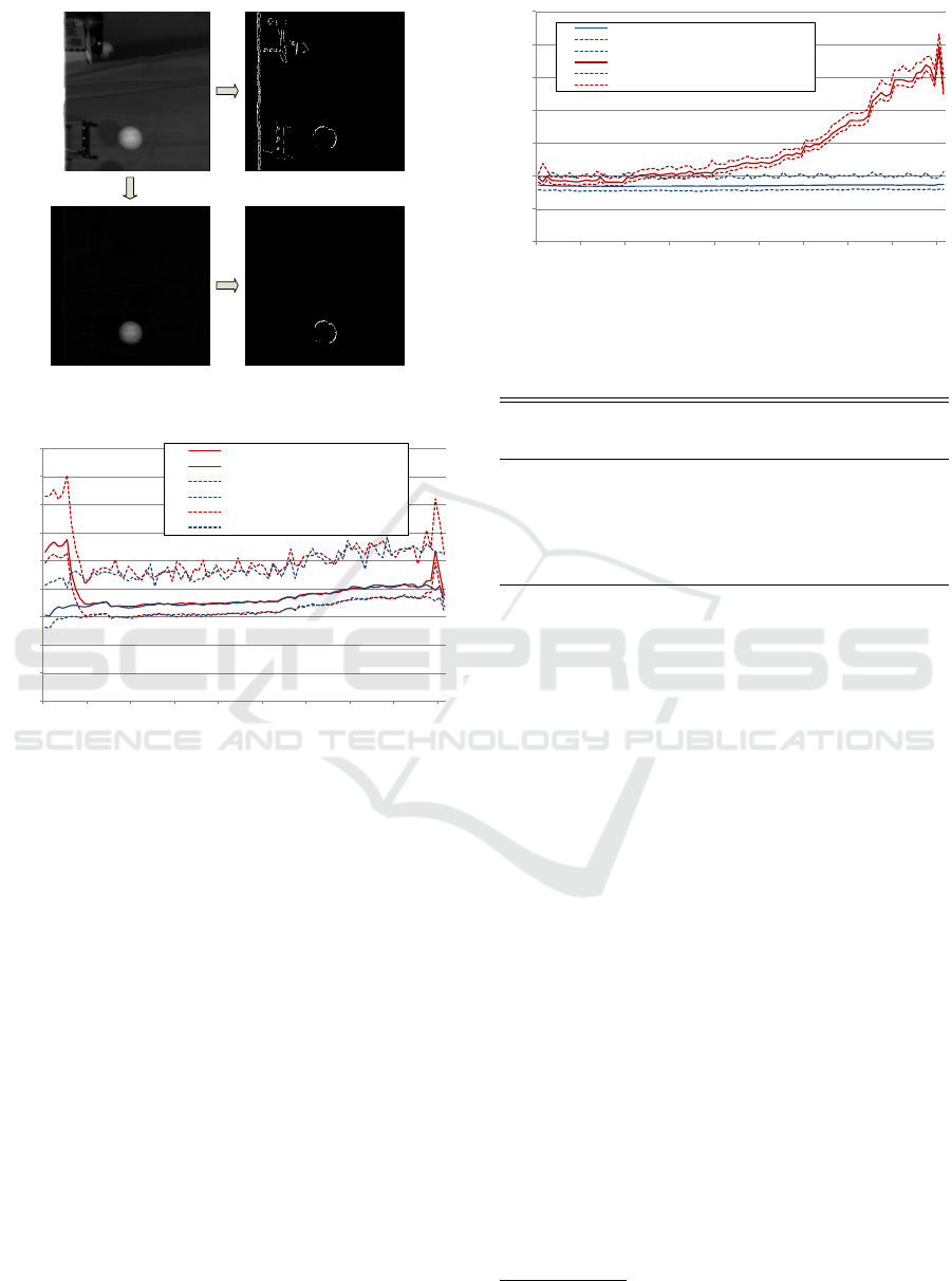
Canny

background

subtraction

Figure 7: The additional step of background subtraction im-

proves an edge image’s quality.

0,5

1,5

2,5

3,5

4,5

1 11 21 31 41 51 61 71 81 91

execution time (ms)

frame number

avg exec time (without bg subtraction)

avg exec time (after bg subtraction)

min exec time (without bg subtraction)

min exec time (after bg subtraction)

max exec time (without bg subtraction)

max exec time (after bg subtraction)

Figure 8: Execution times of background subtraction plus

Canny Edge Detector and of the Canny Edge Detector with-

out a background subtraction.

et al., 2013; Chen et al., 2011). Possibly, they in-

cluded images with a huge amount of edge points, in

which case it might be better to perform the inverse-

checking strategy. The background subtraction af-

fected the Hough Circle Transformation’s execution

times as well: detecting the ball with an untouched

background took up to 2.7× more time than doing this

after the background subtraction step.

Besides, Figure 9 shows that the execution times

of both the Hough Circle Transformation and the

RANSAC algorithm are almost the same at the be-

ginning of the ﬂight when the ball’s image consists in

only a few pixels. Afterward, the RANSAC algorithm

is executing up to 3.4 times faster than the Hough Cir-

cle Transformation.

To obtain reliable statements about the average

tracking error of the determined center point to the

real one, the results of the Hough Circle Transfor-

mation and the RANSAC algorithm were addition-

ally analyzed with the help of the Rauch-TungStriebel

1 11 21 31 41 51 61 71 81 91

execution time (ms)

frame number

avg exec time (RANSAC algorithm)

min exec time (RANSAC algorithm)

max exec time (RANSAC algorithm)

avg exec time (Hough Circle Transformation)

min exec time (Hough Circle Transformation)

max exec time (Hough Circle Transformation)

Figure 9: Execution times of the Hough Circle Transforma-

tion and the RANSAC algorithm for each frame of an entire

ﬂight.

Table 1: Tracking error of ball positioning.

Detection algorithm Background avg. track-

ing error

Hough Circle subtracted 2.73 mm

Hough Circle untouched 25.81 mm

RANSAC subtracted 2.78 mm

RANSAC untouched 25.96 mm

smoother

. This ﬁlter examines the recorded ﬂight

path from front to back and reverse, to create a

smoothed ﬂight path. This smoothing process cor-

rects physically impossible trajectories. Table 1

shows what Figure 7 had already suggested: Subtract-

ing the background considerably improves the detec-

tion’s accuracy as well. In this case, the localized po-

sition is only about 2 to 3mm away from the Rauch-

Tung-Striebel smoother estimated one.

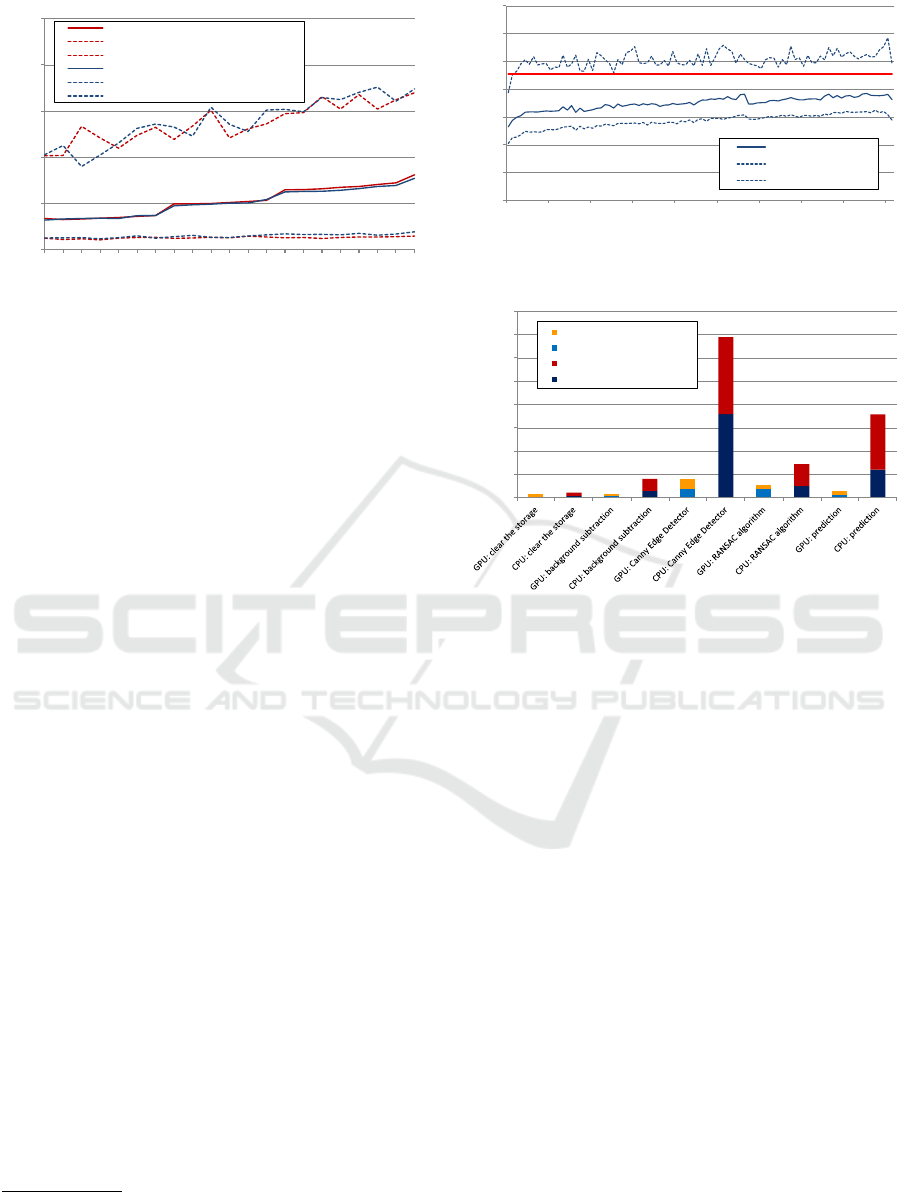
4.3 Prediction

While the accuracy of both prediction algorithms has

been examined earlier (Pongratz, 2016), their execu-

tion times are presented here. Figure 10 shows the

temporal behavior of both methods as functions of

the number of reference trajectories. The average and

minimum time rise fairly linearly as the number of

reference trajectories in the database increases. While

the minimum execution time increases very slowly,

the average time’s graph deﬁnitively illustrates the

impact of including a higher number of reference

throws. This behavior is caused by a larger number

of blocks when more trajectories are in the database.

The temporal behavior of the two approaches is al-

most even, but the time required is slightly different.

While a database with up to 120 trajectories leads to

Available at: http://becs.aalto.ﬁ/en/research/bayes/

ekfukf/

Parallelized Flight Path Prediction using a Graphics Processing Unit

391

0,5

1,5

2,5

1 10 20 30 40 50 60 70 80 90 100 110 120 130 140 150 160 170 180 190 200

execution time (ms)

number of reference trajectories

avg exec time (compare rates of change)

min exec time (compare rates of change)

max exec time (compare rates of change)

avg exec time (compare positions)

min exec time (compare positions)

max exec time (compare positions)

Figure 10: The predictions execution time as a function of

the number of reference trajectories for the comparison of

positions and rates of change.

nearly identical execution times, a small difference

is observed when the number of reference throws in-

creases. For this purpose, the database was ﬁlled with

200 dummy trajectories, all with a length of 92, which

is equivalent to the longest trajectories of an already

existing database. A comparison of the various trials

with different database sizes would not be fair.

4.4 Entire Procedure

The best solution for each step was selected to exam-

ine the execution time of the entire procedure. Each

pair of frames had to run through the following tasks:

clearing the GPU storage, background subtraction,

Canny Edge Detector, RANSAC algorithm, triangu-

lation, coordinate translation, and prediction.

Figure 11 shows the combined execution times of

ﬁve different ﬂights that have been processed 1000

times in a row. The shorter time, as well as the rapid

increase of the time at the beginning of the ﬂight, is

caused by the throwing device, which partially cov-

ered the ball. The slight slope of the graphs is due by

the ball approaching the cameras from frame to frame.

Without our good light proﬁle

, which changes the

Canny Edge Detector’s thresholds in the course of

the ball’s ﬂight, the execution times would signiﬁ-

cantly increase, and the detection would not work that

well. The average maximum time of the different

ﬂights was about 7.69ms and enables a frame rate of

130FPS. Because of maximum execution times that

were, in rare cases, over 10ms, a small buffer is re-

quired for compensation. Without such a buffer, there

would not be sufﬁcient computational power for the

frame rate of 110FPS of the camera system used.

To counteract the heterogeneity of the room’s illumina-

tion (to improve the detection of the ball), we created a light

proﬁle by trial and error.

1 11 21 31 41 51 61 71 81 91

execution time (ms)

frame number

average execution time

minimum execution time

maximum execution time

Figure 11: The execution times of ﬁve ﬂights were pro-

cessed, examined, and combined for this chart.

execution time (ms)

GPU's maximum execution time

GPU's average execution time

CPU's maximum execution time

CPU's average execution time

Figure 12: Average and maximum times of the various tasks

when performing it on a GPU and on a CPU.

For examining the speed-up achieved by using a

GPU instead of a CPU, the entire program was rewrit-

ten to a purely sequential approach on a CPU to be

executable on a CPU. To compare execution times,

one ﬂight was processed 1000 times in a row and the

required times for the various steps were measured.

Figure 12 shows that the largest increase in speed was

measured for the Canny Edge Detector (9.74×) and

the prediction (9.55×), followed by background sub-

traction (5.35×), storage clearing (2.04×), and the

RANSAC algorithm (1.26×). In short, a single frame

was processed 3.46 to 7.17 faster on a GPU than on a

CPU. Hence, this demonstrates that the selected GPU

is a viable platform for this application as it gives a

signiﬁcant performance improvement compared with

the CPU based reference implementation.

Besides the real-time requirement also the track-

ing accuracy of the algorithms is a major concern for

the application. The achieved tracking error, com-

pared to the Rauch-Tung-Striebel smoothened trajec-

tory, was well below 4 cm for 99 % of the tracked

balls over a distance from 0.7 to 3m (Pongratz, 2016).

VISAPP 2017 - International Conference on Computer Vision Theory and Applications

392

5 CONCLUSION

One of the main questions here was whether a GPU

can perform the ball detection and ﬂight path predic-

tion fast enough to achieve a high frame rate. The

results of the NVidia GTX 560 Ti GPU show exe-

cution times that enable data processing at 130FPS.

Moreover, using a GPU for the required calculations

proved to be a beneﬁcial idea. The implemented pro-

gram was 3.46 to 7.17 faster when running on a GPU

than on a CPU; Intel i7-4770S. Using a newer GPU

would - most probably - accelerate the whole pro-

cedure. However, using this ﬁve years old GPU is

representative of GPUs in general. Additionally, as

earlier mentioned, integrated GPUs also offer compu-

tation possibilities. The performance we reached by

using the GPU shows that processing this ﬂight path

prediction will most probably be possible also on an

embedded system with an onboard GPU.

We performed numerous optimizations to enable

such high-speed computation on the GPU used. Well-

thought-out algorithms and letting some data make a

detour over the fast shared memory were the keys to

success. However, some constraints still have to be

considered to achieve an execution time short enough

for this frame rate. Firstly, a small buffer is needed to

compensate for the maximum execution times, which

can be slightly too high for 110FPS (the two cam-

eras captured the scene with 110FPS). Secondly, the

Hough Circle Transformation turned out to be compu-

tationally too costly and time-consuming. Therefore,

the RANSAC algorithm had to be used to achieve the

desired execution time.

Additionally, the background subtraction step and

the adapting threshold proﬁle used for the Canny

Edge Detector were necessary for achieving these ex-

ecution times. Otherwise, a considerably higher num-

ber of edge points would be in the images, which

would lead to an execution time that is too high for

110FPS. These additional computational steps also

enable a more precise detection. For the future, we

plan to consider an approach similar to (Tang et al.,

2015) to use more than one trajectory for the predic-

tion and examine the inﬂuences on the prediction ac-

curacy.

Detecting other - more complex - objects than a

ball will require both more computational power and

more convoluted algorithms. The detection will be

more complicated, and the prediction would have to

take also into account the object’s orientation with its

three degrees of freedom.

REFERENCES

Askari, M. et al. (2013). Parallel gpu implementation of

hough transform for circles. In IJCSI.

Barteit, D. et al. (2009). Measuring the intersection of a

thrown object with a vertical plane. In INDIN.

auml, B. et al. (2011). Catching ﬂying balls and preparing

coffee: Humanoid rollin’justin performs dynamic and

sensitive tasks. In ICRA.

Chen, S. et al. (2011). Accelerating the hough transform

with cuda on graphics processing units. Department

of Computer Science, Arkansas State University.

D’Orazio, T. et al. (2002). A ball detection algorithm for

real soccer image sequences. In ICPR.

Fung, J. et al. (2005). Openvidia: Parallel gpu computer

vision. In ACM Multimedia.

Gowanlock, M. et al. (2015). Indexing of spatiotemporal

trajectories for efﬁcient distance threshold similarity

searches on the gpu. In IPDPS.

Hong, W. et al. (1995). Experiments in hand-eye coordina-

tion using active vision. In Lecture Notes in Control

and Information Sciences.

Jacobs, L. et al. (2013). Object tracking in noisy radar data:

Comparison of hough transform and ransac. In EIT.

Karimi, K. et al. (2010). A performance comparison of

CUDA and opencl. CoRR, abs/1005.2581.

Khronos, G. (2015). Opencl.

Luo, Y. et al. (2008). Canny edge detection on nvidia cuda.

In CVPRW.

NVidia, C. (2014). Cuda architecture.

NVidia, C. (2015). Geforce gtx 560 ti.

Ogawa, K. et al. (2010). Efﬁcient canny edge detection us-

ing a gpu. In ICNC.

Pongratz, M. (2009). Object touchdown position prediction.

Master’s thesis, Vienna University of Technology.

Pongratz, M. (2016). Bio-inspired transport by throwing

system; an analysis of analytical and bio-inspired ap-

proaches. PhD thesis, TU Wien 2016.

Pongratz, M. et al. (2010). Transport by throwing - a bio-

inspired approach. In INDIN.

Pongratz, M. et al. (2012). Koros initiative: Automatized

throwing and catching for material transportation. In

Leveraging Applications of Formal Methods, Veriﬁca-

tion, and Validation, pages 136–143.

Tang, X. et al. (2015). Efﬁcient selection algorithm for fast

k-nn search on gpus. In IPDPS.

Wang, W. et al. (2011). Robust spatial matching for object

retrieval and its parallel implementation on gpu. IEEE

Transactions on Multimedia, 13(6).

Wu, S. et al. (2012). Parallelization research of circle detec-

tion based on hough transform. In IJCSI.

Parallelized Flight Path Prediction using a Graphics Processing Unit

393