Diagnostics of the Arterial Hypertension by Means of the

Discriminant Analysis

Analysis of the Heart Rate Variability Signals Features Combinations

Vladimir Kublanov

, Anton Dolganov

and Yan Kazakov

Research Medical and Biological Engineering Centre of High Technologies, Ural Federal University,

Mira 19, 620002, Yekaterinburg, Russian Federation

Ural State Medical University, Repina 3, 620028, Yekaterinburg, Russian Federation

Keywords: Heart Rate Variability, Arterial Hypertension, Classification, Discriminant Analysis.

Abstract: The paper presents investigation of the diagnostic possibilities of the arterial hypertension using linear and

quadratic combinations of the heart rate variability signals features. For this study, two groups were

considered: healthy volunteers and patients suffering from the arterial hypertension of the II-III degree. For

the study, features of statistical, geometric, spectral, nonlinear and multifractal methods were investigated.

Results of the analysis have shown that among studied combinations four feature sets (heart rate, features of

the VLF frequency band and LF/HF ratio) have the highest classification accuracy – 93%.

1 INTRODUCTION

According to the World Health Organization, arterial

hypertension is among the most common diseases in

the world nowadays. In (Feng et al., 2014) it had been

shown that nearly 40% of people aged 45 years had a

hypertensive disorders. Among the individuals with

hypertension around 40% were unaware of their

condition. In the 2000 there were 972 million people

suffering from the arterial hypertension. According to

current predictions this number will increase to 1,56

billion.

One of the main problems concerning arterial

hypertension is late detection for apparently healthy

people. Therefore, the task of the detection of the

arterial hypertension symptoms is among urgent ones.

The heart rate variability (HRV) signals (R-R

intervals) can be used in this task. Among the

advantages of this signals are safeness, prevalence,

repeatability, ease of the record and relative

cheapness (Kamath et al., 2012).

Studies of the hypertension patients generally use

just couple of statistical and/or spectral features for

the analysis (Scheffler et al., 2013). Most of the

studies devoted to this topic imply analysis of the

long-term Holter monitor (Melillo et al., 2012).

However, for the clinical diagnostics in many cases it

is more appropriate to use short-term signals, about 5

minutes length.

Nowadays, great variety of methods are applied

for the HRVy signals processing: statistical, spectral,

non-linear and multifractal. For the most part, during

one study features of single method are used. As an

example in (Melillo et al., 2014) authors have studied

different features of the non-linear methods for

detecting stress state – Poincare plot, approximate

entropy, correlation dimension and recurrence plot .

On the other hand, there were studies that compares

informativeness of features set of different methods.

In (Ebrahimi et al., 2013) authors have studied 4 sets

of features – time domain features, non-linear

features, discrete wavelet transform features and

empirical mode decomposition features. Results of

that study have shown possibilities of different sets

for automatic sleep staging. However, in that work, as

well as in other known works, the possibilities of each

methods were studied separately and combinations of

features from different methods were not tested.

Application of different methods combination

may increase classification accuracy as incorporation

of various methods data increase informative capacity

of knowledge about the studied object (Wiener,

1961). Because of that, the goal of this work is to

develop methodology of the arterial hypertension

diagnostic by the short-term time series (TS) of HRV

Kublanov V., Dolganov A. and Kazakov Y.

Diagnostics of the Arterial Hypertension by Means of the Discriminant Analysis - Analysis of the Heart Rate Variability Signals Features Combinations.

DOI: 10.5220/0006107902910298

signals using combined estimates, and to study

effectiveness of this methodology.

2 MATERIALS AND METHODS

As the combined estimates in this study, we have used

linear and quadratic combination of two and more

features. Features were obtained by the statistical,

geometric, spectral and multifractal methods. For

evaluation of the diagnostic (classification)

robustness the discriminate analysis have been

applied. All quantifications were performed by the in-

house software developed in MATLAB version

2014b (The MathWorks Inc., Natick, MA).

2.1 Recorded Data

The clinical part of the study was performed in the

Sverdlovsk Clinical Hospital of Mental Diseases for

Military Veterans (Yekaterinburg, Russian

Federation). For the HRV signals registration the

electroencephalograph-analyzer “Encephalan-131-

03” (“Medicom-MTD”, Taganrog, Russian

Federation) was used. The rotating table Lojer

(Vammalan Konepaja DY, Finland) performed the

spatial position change of the patient during passive

orthostatic load – the lift of the head end of the table

was up to 70

from the horizontal position.

Participants of this study: 30 relatively healthy

volunteers and 41 patients suffering from the arterial

hypertension of II and III degree. The signals of HRV

were recorded in two functional states: functional

peace (state F) and passive orthostatic load (state O).

Length of the signal in mentioned state was about 300

seconds.

2.2 Classification

As the classification method, we adopted

discriminant analysis (DA) (Jain, 2010). For this

study, we have trialed linear and quadratic DA.

Linear DA aims to find such linear combination of the

features that can be used for adequate separation

between two classes. In turn, quadratic DA aims to

find quadratic combination of the features for

separation. In case of the current study, two classes

are healthy volunteers and patients with the arterial

hypertension.

Evaluation of the classifiers efficiency was

computed with standard measures for binary

classification performance:

 Total classification accuracy (ACC)



 





;

(1)

 Sensitivity (SEN)

 





;

(2)

 Specificity (SPE)

 





;

(3)

where: P, the total number of patients with arterial

hypertension; N, the total number of healthy

volunteers; TP – True Positive, the number of

correctly classified patients with arterial

hypertension; TN – True Negative, the number of

correctly labelled healthy volunteers; FP – False

Positive, the number of people incorrectly classified

as patients with arterial hypertension; FN – False

Negative, the number of people incorrectly classified

as healthy volunteers (Sokolova and Lapalme, 2009).

For the performance measures evaluation

estimation we adopted 5-fold cross-validation

scheme (Bock et al., 2010). This technique imply

developing five classifiers according to following

steps:

 division of the original dataset randomly into 5

subsamples (i.e. 8 patients for a group with

arterial hypertension and 6 volunteers for

healthy group);

 successive exception of one subsample (testing

subset);

 development of a classifier with the remaining

4 subsamples (training subset);

 testing of classifier with the excluded

subsample;

 computation of the binary classification

measures;

 averaging of the performance measures over 5

classifiers.

Division of the original dataset into 5 subsamples

allowed obtaining person-independent testing.

2.3 Properties of Short-Term HRV

Measures

In this work, we investigated diagnostic possibilities

of the arterial hypertension by the combination of the

different methods of the short-term HRV signals

analysis estimates. Prior to the processing the original

time series were cleaned from the artifacts. By the

artifacts in this study, we considered values of the R-

R intervals that differed from the mean by more than

three values of standard deviation. NN is the

abbreviation for the “normal to normal” time series,

i.e. without artifacts. For spectral and multifractal

analysis NN time series were interpolated using cubic

spline interpolation with the 10 Hz sampling

frequency. Interpolation was performed in MATLAB

software by the interp1 function with method

‘spline’.

2.3.1 Statistical Features

Statistical methods are used for the direct quantitative

evaluation of the HRV time series. Main quantitative

features are:

 M, the mean value of the R-R intervals;

 HR, the Heart Rate, in inverse ration to the M;

 SDNN, the standard deviation of the R-R

intervals;

 CV, the coefficient of variation, defined as ratio

of standard deviation SDNN to the mean M,

expressed in percent;

 RMSSD is the square root of the mean of the

squares of the differences between successive

elements in NN;

 NN5O, the number of pairs of successive

elements in NN that differ by more than 50 ms

(Malik, 1996).

2.3.2 Geometric Features

Geometric methods analyze distribution of the R-R

intervals as a random numbers. The common features

of these methods are:

 М

, the mode, the most frequent value in the R-

R interval. In case of the normal distribution is

close to the mean M;

 VR, the variation range, is the difference

between the lowest R-R interval and the highest

R-R interval in the time series. VR shows

variability of the R-R interval values and

reflects activity of the parasympathetic

department of the autonomic nervous system

(ANS);

 АМ

, the amplitude of the mode, is a number of

the R-R intervals that correspond to the mode

value. AM

shows the stabilizing effect of the

heart rate management, mainly caused by the

sympathetic activity (Malik, 1996).

The following indexes are derived from common

geometric features:

 SI, the Stress Index that reflects centralization

degree of the heart rate and mostly characterize

the activity of the sympathetic department of

the ANS

 

АМ



М



∙

;

(4)

 IAB, the Index of the Autonomic Balance,

depends on the relation between activities of

the sympathetic and parasympathetic

department of the ANS:

 

АМ





; (5)

 ARI, the Autonomic Rhythm Index, which

shows parasympathetic shifts of the autonomic

balance: smaller values of the ARI correspond

to the shift of the autonomic balance to the

parasympathetic activity:



 





∙

;

(6)

 IARP, the Index of Adequate Regulation

Processes, that reflects accordance of the

autonomic function changes of the sinus node

as a reaction of the sympathetic regulatory

effects on the heart

 

АМ



(7)

2.3.3 Spectral Features

Spectral analysis is used to quantify periodic

processes in the heart rate by the means of the Fourier

transform (Fr). The main spectral components of the

HRV signal are High Frequency – HF (0.4 – 0.15 Hz),

Low Frequency – LF (0.15 – 0.04 Hz), Very Low

Frequency – VLF (0.04 – 0.003 Hz), and Ultra Low

Frequency – ULF (lower than 0.003 Hz)

(Malik, 1996). For 300 seconds short-term time series

ULF spectral component is not analyzed.

The studied quantitative features of spectral

analyzes are

 Spectral power of the HF, LF, VLF

components

 Total power of the spectrum – TP;

 Normalized values of the spectral components

by the total power - HF

, LF

and VLF

;

 The LF/HF ratio, also known as the autonomic

balance exponent;

 IC, the Index of centralization

C 





;

(8)

 IAS, the Index of the Subcortical nervous

centers Activation











. (9)

2.3.4 Wavelet Transform

For nonstationary time series one can also use the

wavelet transform (wt), that can simultaneously study

time-frequency patterns. The general equation for

continuous wavelet transform is as follows:





,







√





∙





,

(10)

where:  – the scale, b – the shift , ψ – the wavelet

basis , st – analyzed signal (Addison, 2005).

In MATLAB continuous wavelet transform is

implemented by the cwt function. Moreover, the

connection between the scale and the analyzed

frequency is in accordance with the following:







∗







(11)

where: 



– the central frequency of the wavelet basis,

called by the centfrq function, f

– sampling frequency

of the analyzed signal, f – the analyzed frequency

(Mallat, 2009).

It is possible to acquire same spectral features by

means of the wavelet transform:

 Spectral power of the HF, LF, VLF

components

 Normalized values of the spectral components

by the total power - HF

, LF

and VLF

;

 The LF/HF ratio.

Additionally, standard deviations SDHF(wt),

SDLF(wt), SDVLF(wt) of the HF

(t), LF

(t) and

VLF

(t) TS were tested as features. HF

(t), LF

(t)

and VLF

(t) are TS of the HF, LF and VLF spectral

components respectively, acquired by means of the

wavelet transform.

Moreover, one can study informational

characteristics of the wavelet transform by analyzing

the 









 function. As the features of











 is possible to use number of the

dysfunctions N

, maximal value of the dysfunction

(LF/HF)

max

, and intensity of the dysfunction

(LF/HF)

int

. By the dysfunction, we consider values of

function that suppress decision threshold .

According to our previous studies =10 (Kublanov,

2008). For wavelet transform computation in this

work, we used wavelet Coiflet of the fifth order.

2.3.5 Nonlinear Feature

As the nonlinear feature in this study we have used

the Hurst exponent calculated by the aggregated

variance method. The variance can be written as

followed











































(12)

where H is the Hurst exponent (Rubin et al. 2013).

H can be defined as the slope exponent in the

following equation:

log





∆



log||,

(13)

where 





∆



– is the standard deviation of the ΔХ

increments, corresponding to the time period s, с – the

constant.

Note, that H > 0,5 correspond to the process with

trend, so-called persistent process, contrary H < 0,5

correspond to anti-persistent processes that have a

tendency for trend change, H = 0,5 is the random

process (Mandelbrot, 2003).

2.3.6 Multifractal Features

As the nonlinear method we adopted the multifractal

detrended fluctuation analysis (MFDFA) (Stanley et

al., 1999). Algorithm and application features of the

MFDFA method to estimation of short-term TS are

described in details in (Ihlen, 2012).

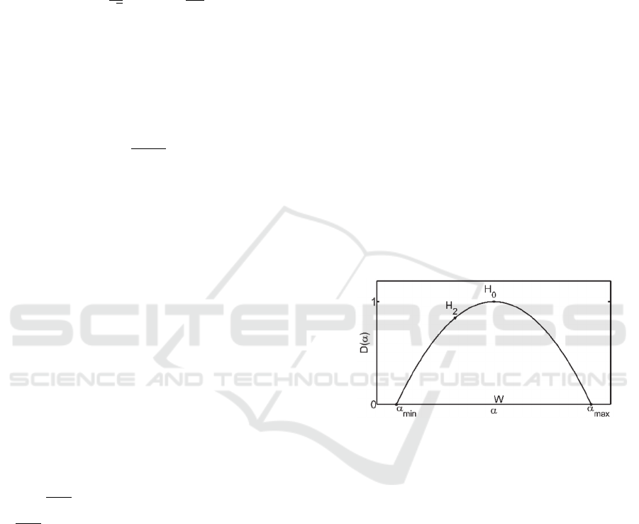
Figure 1: The characteristic features of the multifractal

analysis.

Fig. 1 represents the main features of the

multifractal spectrum estimated by the MFDFA

method. Here, H

is the height of the spectrum,

represents the most probable fluctuations in the

investigated time scale boundary of the signal; H

the generalized Hurst exponent (also known as

correlation degree); 

min

represents behavior of the

smallest fluctuations in the spectrum; 

max

represents

behavior of the greatest fluctuations in the spectrum;

W = 

max

- 

min

, is the width of multifractal spectrum

that shows the variability of fluctuations in the

spectrum. Multifractal characteristics are quantitative

measures of the self-similarity and may characterize

functional changes in the regulatory processes of the

organism.

In addition, we also tested so-called

1/2

width

measure of the spectrum, which is defined as

1/2

=|H

-H

| (Makowiec et al., 2011)

In this study, we investigated time scale

boundaries that correspond to the LF and VLF

frequency bands: (6-25) sec and (25-300) sec

respectively. In our earlier works and by other authors

it was noted that multifractal analysis of the HF

component is not informative because of the noising,

(Makowiec et al., 2012).

3 RESULTS AND DISCUSSION

In this study, we wanted to test all possible

combinations of the features. However, the number of

k-combinations of 53 features is quite high for k

equaled to 2, 3 and 4 - 1378, 23426 and 292825,

respectively. In order to decrease computation time

and remove redundant results (formed by the features

that are already combination of previous features) we

have decided to use for further test only those

combinations that are formed by non-correlated

features.

The correlation coefficient was calculated in

MATLAB software by the corrcoef function. The

threshold for the correlation coefficient was set to be

lower than 0,25. Using this threshold number of

combination was reduced to 629 for two features

combinations, to 1985 for three features combinations

and to 1995 for four features combinations.

3.1 Single Feature Test

For the F state none of the tested features showed

ACC higher than 75 %. The best results of the

classification efficiency estimation for the state O are

presented in table 1. Another 8 combinations have

ACC higher than 76%.

Table 1: Efficiency of the classification for the linear DA

for state O of the single features, %.

feature SEN SPE ACC

VLF

90 73 83

VLFn(Fr)

83 76 80

VLFn(wt)

85 73 80

According to the data shown in table 6 one can

conclude that application of the single feature

for the arterial hypertension classification is

not sufficient. Therefore, application of two

and more features combinations is justified.

3.2 Two Features Combination Test

Three combinations of features combinations (M and

VLFn(wt),VLFn(Fr) and VLF(wt), VLFn(Fr) and

SDVLF(wt)) for the signals recorded in state F

obtained by the linear DA. achieved the highest

results (ACC 77%). Another 14 combinations that are

formed by the statistical and spectral features, have

ACC not less than 75 %.

Table 2 presents the highest results of the

classification efficiency for two features

combinations of the signals recorded in state O

obtained by the linear DA. Another 42 combinations

that are formed by the statistical, spectral and

multifractal features have ACC not less than 80 %.

Table 2: Efficiency of the classification for the linear DA

for state O of the two feature combinations, %.

features SEN SPE ACC

HFn(Fr), W

1/2

LF 95 73 86

VLFn(Fr), LF/HF(Fr) 93 76 86

VLFn(Fr), LF/HF(wt) 93 76 86

VLFn(Fr), H 95 73 86

LF/HF(Fr), VLFn(wt) 93 76 86

HFn(wt), W

1/2

LF 95 73 86

VLFn(wt), LF/HF(wt) 93 76 86

VLFn(wt), H 93 76 86

Two combinations of features (VLFn(Fr) and

LF/HF(Fr), VLFn(wt) and H) for the signals recorded

in state F obtained by the quadratic DA achieved the

highest results (ACC 76%).

Table 3 presents the highest results of the

classification efficiency for two features

combinations of the signals recorded in state O

obtained by the quadratic DA. Another 42

combinations that are formed by the statistical,

spectral and multifractal features have ACC not less

than 80 %.

According to the data presented in tables 2-3 one

can conclude:

 features of the signals recorded in state O allows

to reach higher classification results than those

recorded in state F;

 for two features combinations the highest results

are obtained by combinations of the spectral and

multifractal features;

 application of two features combination improves

classification efficiency compared to application

of single feature, however it is not possible to

achieve simultaneously high specificity and

sensitivity.

Table 3: Efficiency of the classification for the linear DA

for state O of the two feature combinations, %.

features SEN SPE ACC

VLFn(Fr), H 95 73 86

LF/HF(Fr), VLFn(wt) 88 83 86

HR, H2 VLF 93 73 84

VLFn(Fr), SDVLF(wt) 88 79 84

VLFn(Fr), LF/HF(wt) 83 86 84

VLFn(Fr), (LF/HF)

max

85 83 84

SDVLF(wt), VLFn(wt) 90 76 84

VLFn(wt), LF/HF(wt) 85 83 84

VLFn(wt), W

1/2

LF 88 80 84

VLFn(wt), H 93 73 84

3.3 Three Features Combination Test

The highest result of the classification efficiency for

the signals recorded in state F obtained by the linear

DA was achieved by the combination of M0,

(LF/HF)max, H2 VLF (ACC 78%). Another 17

combinations that are formed by the statistical,

spectral and multifractal features have ACC not less

than 77 %.

Table 4 presents the highest results of the

classification efficiency for three features

combinations of the signals recorded in state O

obtained by the linear DA. Another 83 combinations

that are formed by the statistical, spectral and

multifractal features have ACC not less than 85 %,

while having SPE and SEN not less than 75 %.

Table 4: Efficiency of the classification for the linear DA

for state O of the three feature combinations, %.

features SEN SPE ACC

HR, VLFn(Fr), H

LF 95

87 91

VLFn(Fr), LF/HF(Fr), W

1/2

LF 93 87 90

VLFn(Fr), LF/HF(wt), W

1/2

LF 93 87 90

VLFn(Fr), (LF/HF)int, W

1/2

LF 93 87 90

The highest result of the classification efficiency

for the signals recorded in state F obtained by the

quadratic DA was achieved by three combinations

(VLFn(Fr), (LF/HF)int, H; VLFn(wt), (LF/HF)int, H;

VLFn(wt), H0 LF, H) with ACC 77%.

Table 5 presents the highest results of the

classification efficiency for three features

combinations of the signals recorded in state O

obtained by the quadratic DA. Another 65

combinations that are formed by the statistical,

spectral and multifractal features have ACC not less

than 85 %, while having SPE and SEN not less than

75 %.

Table 5: Efficiency of the classification for the quadratic

DA for state O of the three feature combinations, %.

features SEN SPE ACC

LF/HF(Fr), SDVLF(wt),

VLFn(wt)

89 90

SDVLF(wt), VLFn(wt),

LF/HF(wt)

90 89 90

HR, VLFn(Fr), SDVLF(wt) 85 93 89

VLFn(Fr), LF/HF(Fr),

VLF(wt)

88 89 89

VLFn(Fr), LF/HF(Fr),

SDVLF(wt)

88 89 89

VLFn(Fr), LF/HF(Fr), W

1/2

90 87 89

VLFn(Fr), VLF(wt),

LF/HF(wt)

88 89 89

VLFn(Fr), (LF/HF)

max

, W

VLF

93 83 89

LF/HF(Fr), VLFn(wt), W

1/2

90 87 89

SDVLF(wt), VLFn(wt),

(LF/HF)

int

93 83 89

VLFn(wt), (LF/HF)

max

, W

VLF

90 87 89

According to the data presented in tables 4-5 one

can conclude:

 features of the signals recorded in state O allows

to reach higher classification results than those

recorded in state F, same result as for two feature

combinations;

 for three features combinations the highest results

are obtained by combinations of the spectral

features as well as combination of spectral,

statistic and multifractal features;

 application of three features combination

improves classification efficiency compared to

application of two features combination, it is

possible to achieve high accuracy (more than 90

%), while maintaining high level of specificity(up

to 89 %) and sensitivity (up to 95 %).

3.4 Four Features Combination Test

Five feature combinations of the signals recorded in

state F obtained by the linear DA (IAB, IAS,

(LF/HF)int, W1/2 VLF; VLF(Fr), IAS, LF/HF(wt),



max

VLF; LF/HF(Fr), IAS, VLF(wt), 

max

VLF; IAS,

VLF(wt), LF/HF(wt),



max

VLF; HF(wt), (LF/HF)int,

H2 VLF, H) achieved the highest results of the

classification efficiency (ACC 79%). Another 27

combinations that are formed by the statistical,

spectral and multifractal features have ACC not less

than 77 %.

Table 6 presents the highest results of the

classification efficiency for four features

combinations of the signals recorded in state O

obtained by the linear DA. Another 93 combinations

that are formed by the statistical, spectral and

multifractal features have ACC not less than 85 %,

while having SPE and SEN not less than 75 %.

Table 6: Efficiency of the classification for the linear DA

for state O of the four feature combinations, %.

features SEN SPE ACC

HR, VLFn(Fr), VLF(wt),

(LF/HF)

max

90 93 91

HR, SDVLF(wt),

VLFn(wt), (LF/HF)

max

90 93 91

HR, VLFn(Fr),

SDVLF(wt), (LF/HF)

max

87 93 90

HR, VLF(wt), VLFn(wt),

(LF/HF)

max

90 90 90

Three feature combinations for the signals

recorded in state F obtained by the quadratic DA

(ARI, IAS, Nd, W1/2, VLF; ARI, IAS, (LF/HF)int,

W1/2 VLF; VLFn(Fr), (LF/HF)max,



min

LF, W1/2

VLF) achieved the highest classification efficacy

(ACC > 75%).

Table 7 presents the highest results of the

classification efficiency for four features

combinations of the signals recorded in state O

obtained by the quadratic DA. Another 77

combinations that are formed by the statistical,

spectral and multifractal features have ACC not less

than 85 %, while having SPE and SEN not less than

75 %.

Table 7: Efficiency of the classification for the quadratic

DA for state O of the four feature combinations, %.

features SEN SPE ACC

HR, SDVLF(wt), VLFn(wt),

(LF/HF)

max

93 93

HR, VLFn(Fr), SDVLF(wt),

(LF/HF)

max

93 90 91

M, VLFn(Fr), VLF(wt),

(LF/HF)

max

93 86 90

HR, VLFn(Fr), VLF(wt),

(LF/HF)

max

90 90 90

HR, VLF(wt), VLFn(wt),

(LF/HF)

max

90 90 90

VLF(Fr), VLFn(Fr), (LF/HF)

int

W VLF

93 87 90

According to the data presented in tables 6-7 one

can conclude:

 features of the signals recorded in state O allows

to reach higher classification results than those

recorded in state F, same result as for two and

three feature combinations;

 for four features combinations the highest results

are obtained by combinations statistical features

HR and M and spectral features;

 application of four features combination further

improves classification efficiency compared to

application of three features combination; it is

possible to achieve relatively high accuracy,

specificity, sensitivity; the specific combinations

of HR and spectral features achieves ACC, SPE

and SEN, all higher than 90 %.

4 CONCLUSIONS

The paper described results of the diagnostic

possibilities test of statistic, geometric, spectral, non-

linear and multifractal features for discrimination of

the arterial hypertension.

Obtained results have shown that classification

efficiency increases as number of features in

combination increases. For four features

combination, formed by HR, VLF estimates and

LF/HF ratio, accuracy, sensitivity and specificity

suppress 90%. Linear and quadratic DA have shown

about the same results of the classifier efficiency.

Results of the current study have higher

classification efficiency compared to our previous

works. There we analyzed comparable sample of

subjects, using single feature in two-dimensional

space: “state F – state O” (Kublanov et al., 2016).

Furthermore, current results suppress classification

efficacy of some other authors. In particular results of

the Artificial Neural Network and Logistic

Regression Analysis models for patients with

hypertension (Tang et al., 2013).

In our opinion this results confirms scientists’

interpretation of the arterial hypertension

development mechanisms. The activation of the

sympathetic nervous system takes important part in

the initialization of the arterial hypertension,

maintenance of the increased vascular tone as well as

increased cardiac output. Role of the vascular system

regulation central mechanisms disorders, including

lost balance of suprasegmental autonomic regulation

and development of the anxiety and depression

disorders (Parati and Esler, 2012, 2013 ESH/ESC

guidelines for the management of arterial

hypertension, 2013).

Results of our study shows application

possibilities of the combined estimates of the short-

term time series heart rate variability signals for the

arterial hypertension diagnostics. In future works, our

research group will continue study this problem on

larger sample of subjects in order to improve

robustness of the classification as well as compare

discriminate analysis performance versus other

methods on the same sample of subjects.

ACKNOWLEDGEMENTS

The work was supported by Act 211 Government of

the Russian Federation, contract № 02.A03.21.0006.

REFERENCES

2013 ESH/ESC guidelines for the management of arterial

hypertension: The Task Force for the management of

arterial hypertension of the European Society of

Hypertension (ESH) and of the European Society of

Cardiology (ESC), 2013. European Heart Journal, 34

(28), 2159–2219.

Bock, R., Meier, J., Nyúl, L.G., Hornegger, J., and

Michelson, G., 2010. Glaucoma risk index: Automated

glaucoma detection from color fundus images. Medical

Image Analysis, 14 (3), 471–481.

Ebrahimi, F., Setarehdan, S.-K., Ayala-Moyeda, J., and

Nazeran, H., 2013. Automatic sleep staging using

empirical mode decomposition, discrete wavelet

transform, time-domain, and nonlinear dynamics

features of heart rate variability signals. Computer

Methods and Programs in Biomedicine, 112 (1), 47–57.

Feng, X.L., Pang, M., and Beard, J., 2014. Health system

strengthening and hypertension awareness, treatment

and control: Data from the China health and retirement

longitudinal study. Bulletin of the World Health

Organization, 92 (1), 29–41.

Ihlen, E.A.F., 2012. Introduction to multifractal detrended

fluctuation analysis in Matlab. Frontiers in Physiology,

3 JUN.

Jain, A.K., 2010. Data clustering: 50 years beyond K-

means. Pattern Recognition Letters, 31 (8), 651–666.

Kamath, M.V., Watanabe, M., and Upton, A., 2012. Heart

Rate Variability (HRV) Signal Analysis: Clinical

Applications. New York: CRC Press.

Kublanov, V., Dolganov, A., and Borisov, V., 2016.

Application of the Discriminant Analysis for

Diagnostics of the Arterial Hypertension - Analysis of

Short-Term Heart Rate Variability Signals. Presented at

the 4th International Congress on Neurotechnology,

Electronics and Informatics, 45–52.

Kublanov, V.S., 2008. A hardware-software system for

diagnosis and correction of autonomic dysfunctions.

Biomedical Engineering, 42 (4), 206–212.

Makowiec, D., Rynkiewicz, A., Gałaska, R., Wdowczyk-

Szulc, J., and Żarczyńska-Buchowiecka, M., 2011.

Reading multifractal spectra: Aging by multifractal

analysis of heart rate. EPL (Europhysics Letters), 94

(6), 68005.

Makowiec, D., Rynkiewicz, A., Wdowczyk-Szulc, J., and

Zarczynska-Buchowiecka, M., 2012. On reading

multifractal spectra. multifractal age for healthy aging

humans by analysis of cardiac interbeat time intervals.

Acta Physica Polonica B, Proceedings Supplement, 5

(1), 159–170.

Malik, M., 1996. Heart rate variability: Standards of

measurement, physiological interpretation, and clinical

use. Circulation, 93 (5), 1043–1065.

Mallat, S., 2009. A Wavelet Tour of Signal Processing.

Mandelbrot, B.B., 2003. Multifractal Power Law

Distributions: Negative and Critical Dimensions and

Other ‘Anomalies,’ Explained by a Simple Example.

Journal of Statistical Physics, 110 (3–6), 739–774.

Melillo, P., Izzo, R., De, L., and Pecchia, L., 2012. Heart

rate variability and target organ damage in hypertensive

patients.

BMC Cardiovascular Disorders, 12.

Melillo, P., Pacifici, E., Orrico, A., Iadanza, E., and

Pecchia, L., 2014. Heart rate variability for automatic

assessment of congestive heart failure severity. IFMBE

Proceedings, 41, 1342–1345.

Parati, G. and Esler, M., 2012. The human sympathetic

nervous system: Its relevance in hypertension and heart

failure. European Heart Journal, 33 (9), 1058–1066.

Rubin, D., Fekete, T., and Mujica-Parodi, L.R., 2013.

Optimizing Complexity Measures for fMRI Data:

Algorithm, Artifact, and Sensitivity. PLoS ONE, 8 (5).

Scheffler, P., Muccio, S., Egiziano, G., Doonan, R.J., Yu,

A., Carli, F., and Daskalopoulou, S.S., 2013. Heart rate

variability exhibits complication-dependent changes

postsurgery. Angiology, 64 (8), 597–603.

Sokolova, M. and Lapalme, G., 2009. A systematic analysis

of performance measures for classification tasks.

Information Processing and Management, 45 (4), 427–

437.

Stanley, H.E., Amaral, L.A.N., Goldberger, A.L., Havlin,

S., Ivanov, P.C., and Peng, C.-K., 1999. Statistical

physics and physiology: Monofractal and multifractal

approaches. Physica A: Statistical Mechanics and its

Applications, 270 (1–2), 309–324.

Tang, Z.-H., Liu, J., Zeng, F., Li, Z., Yu, X., and Zhou, L.,

2013. Comparison of Prediction Model for

Cardiovascular Autonomic Dysfunction Using

Artificial Neural Network and Logistic Regression

Analysis. PLoS ONE, 8 (8).

Wiener, N., 1961. Cybernetics Or Control and

Communication in the Animal and the Machine. MIT

Press.