Improving Bayesian Mixture Models for Colour Image Segmentation

with Superpixels

Thorsten Wilhelm and Christian W

ohler

Image Analysis Group, TU Dortmund, Otto-Hahn Str. 4, Dortmund, Germany

Keywords:

Bayesian, MCMC, Mixture Models, Segmentation, Superpixel, Texture.

Abstract:

The large computational demand is one huge drawback of Bayesian Mixture Models in image segmentation

tasks. We describe a novel approach to reduce the computational demand in this scenario and increase the per-

formance by using superpixels. Superpixels provide a natural approach to the reduction of the computational

complexity and to build a texture model in the image domain. Instead of relying on a Gaussian mixture model

as segmentation model, we propose to use a more robust model: a mixture of multiple scaled t-distributions.

The parameters of the novel mixture model are estimated with Markov chain Monte Carlo in order to surpass

local minima during estimation and to gain insight into the uncertainty of the resulting segmentation. Finally,

an evaluation of the proposed segmentation is performed on the publicly available Berkeley Segmentation

database (BSD500), compared to competing methods, and the beneﬁt of including texture is emphasised.

1 INTRODUCTION

Image segmentation techniques are required in many

computer vision applications. Dividing an image into

coherent regions, which are possibly close to human

perception is not a trivial task. Compression artefacts,

shading, occlusion, and cluttered and textured regions

hinder a simple colour based approach from working

well. Further, the number of possible solutions is ac-

tually quite large and can be computed by the Stirling

partition number (Graham et al., 1994). In the case

of n = 10 data points and k = 3 clusters already 9330

possible clusterings arise.

Generative models are one way among many oth-

ers to divide an image or a set of data points into

meaningful clusters. Our focus resides on genera-

tive models because they offer a way to describe and

model the properties of different regions in a coherent

framework. This is not straightforward in discrimi-

native models, which additionally require a large por-

tion of supervision to work well. In generative mod-

elling the underlying probability distribution which

generated the data is attempted to be approximated

by a model. Commonly, mixture models are used.

One frequent representative of this type of model is

the Gaussian mixture model (GMM), which is usu-

ally estimated by a technique based on the Expecta-

tion Maximisation algorithm (EM) (Dempster et al.,

1977). However, EM tends to be subject to local

minima (McLachlan and Krishnan, 2007). Bayesian

methods provide a good alternative. Through intro-

ducing prior distributions and trying to estimate the

underlying probability distribution of the parameters

instead of single point estimates, local minima may

be left, because during the sampling of the Markov

chain values with a lower probability than the cur-

rent estimate are accepted. The sampling process

leads to an increase of the computational demands,

because in every iteration the whole model needs to

be evaluated. As a result, the statistical literature of-

fers several ways to reduce the computational demand

of Bayesian methods.

Segmentation in general is a task where a large

number of data points have to be considered, because

one image usually consists of millions to billions of

data points depending on the resolution of the image.

The statistics literature focuses on favourable ways to

approximate the posterior distribution as accurately as

possible, although the number of data points is re-

duced during parameter estimation. This is for in-

stance achieved by subsampling of the data points for

likelihood evaluation (Korattikara et al., 2013; Bar-

denet et al., 2014) or by relying on the computation of

lower bounds (Maclaurin and Adams, 2014). We pro-

pose instead to use a domain speciﬁc approximation

technique to vastly reduce the computational demand,

namely superpixels. Superpixels are a description of

local neighbourhoods and can therefore directly be

Wilhelm T. and WÃ˝uhler C.

Improving Bayesian Mixture Models for Colour Image Segmentation with Superpixels.

DOI: 10.5220/0006111504430450

In Proceedings of the 12th International Joint Conference on Computer Vision, Imaging and Computer Graphics Theory and Applications (VISIGRAPP 2017), pages 443-450

ISBN: 978-989-758-225-7

443

used to build an additional texture model of the im-

age (see Section 3) .

2 RELATED WORK

Superpixels are a commonly used pre-processing step

in computer vision and are applied in a large variety

of computer vision tasks. This includes, among oth-

ers, segmentation (Achanta et al., 2012), object detec-

tion (Fulkerson et al., 2009), medical image analysis

(Cheng et al., 2013), and hyperspectral image analysis

(Thompson et al., 2010). While the origin of super-

pixels dates back to (Ren and Malik, 2003), research

has developed in several ways to estimate superpixels

from an image. This includes gradient or graph based

methods, or methods based on a k-means clustering.

See (Achanta et al., 2012) for an overview.

The superpixel representation has several beneﬁts

over other techniques which aim to reduce the com-

putational expenses in image analysis. For instance,

if uniform sub-sampling of the image is performed,

information is lost and a ﬁltering is required to reduce

sampling artefacts. By looking at small rectangular

regions of an image, the borders of different regions

or objects usually do not coincide with the rectangu-

lar regions. In contrast, superpixels aim to preserve

the structure of an image by ﬁnding small coherent

regions.

2.1 Morphological Reconstruction

While superpixels are a way to reduce the over-

all amount of data points in a useful manner, other

pre-processing steps may be included in the analy-

sis pipeline to modify the data in a beneﬁcial way.

Morphological reconstruction (Vincent, 1993) is one

of such techniques and can be applied to binary and

grey scale images. In the binary case morphological

reconstruction computes connected components and

in the grey scale case it is used to remove local peaks

from the distribution of pixel intensities. Morpho-

logical reconstruction aims to reconstruct the image

I from a marker image M. As a result, local peaks

are removed from the image by subsequent dilation of

M constrained through I. The marker image is con-

structed by erosion with a structuring element S. In

our case S is disk-shaped with radius S

According to (Benesova and Kottman, 2014) we

apply morphological reconstruction six times using a

marker image, which is computed by eroding the orig-

inal image with a disk of size S

= s px. Once for

every colour channel and once for the inverse of ev-

ery colour channel, removing local light and dark ex-

tremes from the image. The advantage of this prepro-

cessing step is that it preserves edges between neigh-

bouring regions, while additionally removing high

frequency patterns from the image, which aids the

mixture model in modelling the structure of the im-

age. An analysis of the effect of this operation is

provided in the experiments section. The effect of

morphological reconstruction with various sizes of

the eroding disk is illustrated in Figure 1. Note how

the eyes of the koala gradually vanish with increasing

disk size.

2.2 Texture Features

Various texture features have been proposed in the lit-

erature. This includes, among others, Textons (Ar-

belaez et al., 2011), grey-level-co-occurrence matri-

ces and Haralick features, (Haralick et al., 1973),

Laws’ texture energy features (Laws, 1980), dense

SIFT (Tighe and Lazebnik, 2013), windowed second

moment matrices of a local neighbourhood (Belongie

et al., 1998), dictionary learning using k-means (Dahl

and Dahl, 2015), structured tensors (Rousson et al.,

2003), and histogram based methods (Kim et al.,

2005). While all methods look at a local neighbour-

hood around a pixel to deﬁne a measure of texture,

not all methods are directly compatible with super-

pixels, because they look at rectangular regions like

Textons or simply do not match the superpixel size,

like dense SIFT. Textons yield another difﬁculty, be-

cause the most meaningful ﬁlters occur around the

edges of neighbouring regions, which makes it difﬁ-

cult to use them to distinguish between different tex-

tures. Since our goal is to include a single texture

feature into the mixture model we propose a custom

texture map based on histograms and a superpixel rep-

resentation of the image. Therefore it accounts for the

superpixel borders, is one-dimensional, and it is de-

ﬁned in an euclidean space, which makes it suitable

to be integrated as another dimension in a generative

model (cf. Section 3).

2.3 Choice of Mixture Distribution

Commonly, images are modelled as Gaussian Mix-

tures. However, in practice outliers frequently occur

and a Gaussian distribution is not necessarily an ap-

propriate description of every part of the image. This

either leads to over-segmentations or an incoherent

segmentation of the image. One possibility to in-

crease the ﬂexibility of the mixture model is to change

the mixture distribution to something different from

the Gaussian distribution. (Nguyen and Wu, 2012)

use a multivariate t-distribution, and (Wilhelm and

VISAPP 2017 - International Conference on Computer Vision Theory and Applications

444

Raw Image

= 2 px S

= 5 px S

= 7 px S

= 9 px

Figure 1: Effect of the extent S

of the eroding disk during morphological reconstruction. Image taken from the validation set

of the BSD500 (Arbelaez et al., 2011).

ohler, 2016) use a generalised hyperbolic distribu-

tion (GHD). While the use of a GHD is generally jus-

tiﬁed if a huge number of data points is available, for

superpixels, which aim to efﬁciently reduce the num-

ber of data points, the sample size may be to small too

achieve meaningful parameter estimates. However, a

robust distribution seems favourable in the task of im-

age segmentation. Therefore we propose to use a mul-

tiple scaled variant of the multivariate t-distribution

(Forbes and Wraith, 2014). The probability density

function (pdf) of the multivariate t-distribution corre-

sponds to

t(x|µ

µ,Σ

Σ,ν) =

Γ((ν + p)/2)

Γ(ν/2)ν

p/2

1/2



1 +

(x − µ

µ)

−1

(x − µ

µ)



(1)

with the number of degrees of freedom ν, the num-

ber of dimensions p, the mean vector µ

µ, and the co-

variance matrix Σ

Σ. The parameter ν describes the

tail behaviour of the distribution. This enables the

distribution to place more weight on infrequent data

points and as a result achieve robust estimates of the

parameters in comparison to a Gaussian distribution.

Since the tail behaviour is equal in every dimension

this enforces a rather strict assumption on the shape

of the distribution. One can easily imagine cases

where this shape may not be desired. We therefore

choose the multiple scaled variant of the multivariate

t-distribution (Forbes and Wraith, 2014) as the model

for a single component of the mixture model. In con-

trast to a multivariate t-distribution the multiple scaled

variant allows to set the scale parameter ν indepen-

dently for every dimension, including the unscaled

variant if ν is equal in every dimension. According

to (Tortora et al., 2014) the pdf is

(x|µ

µ,Γ

Γ,Φ

Φ,ν

ν) =

∏

j=1

Γ((ν

+ 1)/2)

Γ(ν

/2)(Φ

π)

1/2





1 +



[x − µ

µ]







−(ν

+1)/2

(2)

with mean vector µ

µ, the eigenvectors Γ

Γ and eigenval-

ues Φ

Φ of Σ

Σ, and ν

ν the vector of degrees of freedoms.

We use this distribution, because it is a compromise

between ﬂexibility and simplicity. Further details on

the distribution may be found in (Forbes and Wraith,

2014) or (Tortora et al., 2014).

2.4 Delayed Rejection Adaptive

Metropolis

Estimation of the model is performed in a Bayesian

framework, because it enables us to aid the mix-

ture model by deﬁning appropriate prior distributions

for the model parameters. Recall, in a Bayesian

framework the model parameters are not point esti-

mates, but probability distributions and the parame-

ters of these distributions are usually estimated with

Markov chain Monte Carlo (MCMC). One of such al-

gorithms which performs this is Metropolis-Hastings

(MH) (Hastings, 1970), which is described by (Nt-

zoufras, 2011) as follows:

1. Initialise θ

(0)

2. For t = 1,...,T

(a) Set θ

θ = θ

(t−1)

(b) Obtain new candidate parameter using the pro-

posal distribution q(θ → θ

) = q(θ

|θ).

α = min



p(θ

|X)q(θ

θ|θ

)

p(θ

θ|X)q(θ

|θ

θ)



= min (1,A).

(3)

(d) Update θ

(t)

= θ

with probability α, otherwise

set θ

(t)

= θ

θ = θ

(t−1)

Improving Bayesian Mixture Models for Colour Image Segmentation with Superpixels

445

In contrast to a common MH step, Delayed Re-

jection Adaptive Metropolis (DRAM) (Haario et al.,

2006) aims to improve the exploration and conver-

gence speed of the Markov chain by adapting the

proposal distribution q(θ → θ

) on the ﬂy. In con-

trast to other methods, which compute the gradient of

the posterior, like Hamiltonian Monte Carlo (HMC)

(Hoffman and Gelman, 2014) DRAM does not need

to evaluate the gradient of the posterior distribu-

tion. Actually DRAM combines two separate tech-

niques, Delayed Rejection (DR) (Tierney and Mira,

1999) and Adaptive Metropolis (AM) (Haario et al.,

2001). While DR does not afﬂict the assumptions of

a Markov chain, AM violates them and the resulting

chain is neither Markovian nor reversible. However,

in practice this does not always seem to inﬂuence the

results strongly and can even be beneﬁcial (Haario

et al., 2006), because it improves the exploration of

the parameter space. This is especially beneﬁcial in

high dimensional parameter spaces, where it is difﬁ-

cult to design appropriate multivariate proposal distri-

butions.

Delayed Rejection works as follows. In contrast to

a common MH step, where the proposal move is ei-

ther accepted or rejected, DR modiﬁes this behaviour

by not wasting this information, but by proposing a

new sample, which can be based on a different pro-

posal distribution or on the rejected sample itself.

This delaying may be iterated several times, for in-

stance based on a ﬁxed number or on deﬁned proba-

bility.

AM modiﬁes the proposal distribution of the MH

step during the sampling by determining the empiri-

cal covariance of the chain and using this information

to propose new samples for the MH acceptance step.

This violates the assumptions of the Markov chain,

yet it works in practice. Further details on DRAM

may be found in (Haario et al., 2006).

2.5 Accuracy Evaluation of

Segmentation Tasks

After the model is estimated, an evaluation of the re-

sult is important in order to compare it to different

approaches. Commonly two ways exist to evaluate

the accuracy of the segmentation. The ﬁrst variant

looks at the boundaries of the segments and treats the

segmentation as a binary classiﬁcation problem. See

(Arbelaez et al., 2011) for further details. The other

way is to look at the segmentation itself and mea-

sure the accuracy of the underlying clustering. Two

commonly used quantities are the Probabilistic Rand

Index (PRI) and the Variation of Information (VoI).

The PRI between a computed segmentation A and a

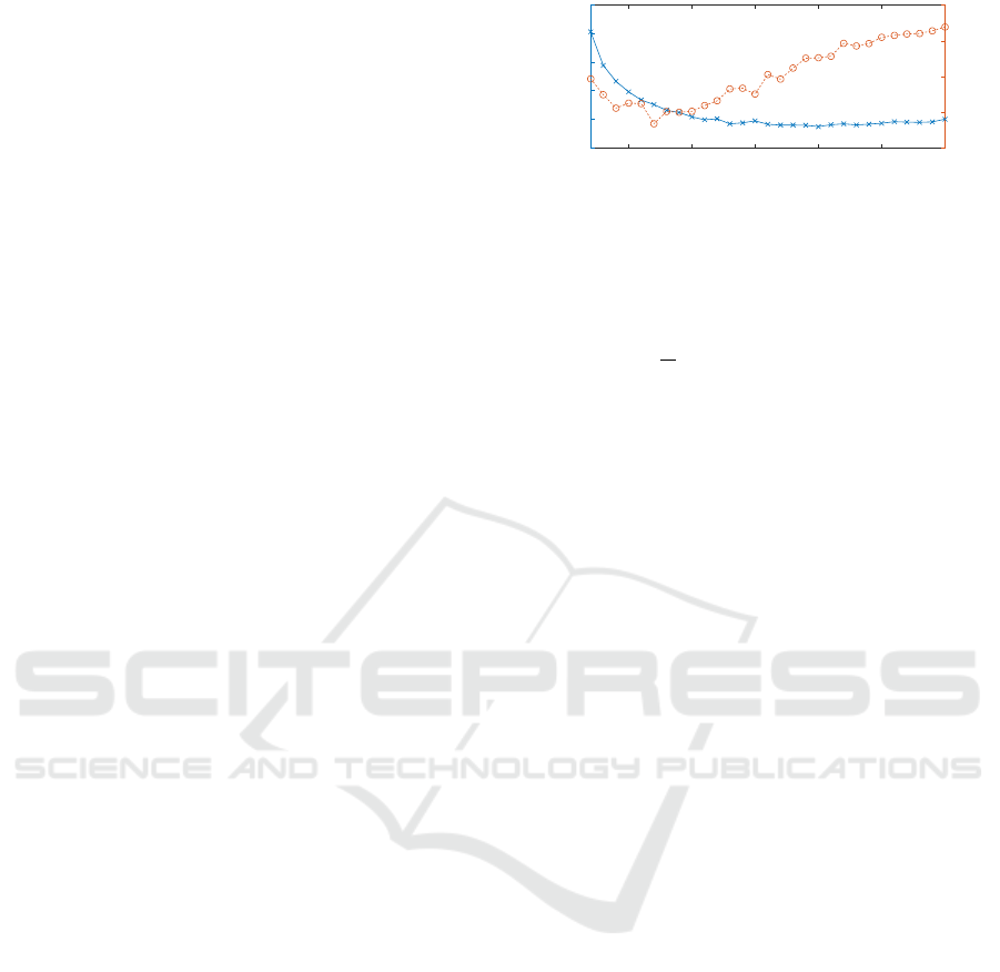
5 10 15 20 25 30

# Components

2000

4000

6000

8000

10000

BIC [-]

1.5

2.5

VoI [-]

Figure 2: Relation between BIC and VoI for the image used

in Figure 3.

ground-truth segmentation G is deﬁned by (Arbelaez

et al., 2011) as

PRI(A,G) =

∑

i< j

i j

+ (1 − ci j)(1 − pi j)], (4)

where c

i j

indicates if pixel i and j have identical labels

and p

i j

is the corresponding probability of this event.

VI measures the difference in terms of the average

conditional entropy between segmentations A and G,

deﬁned by (Arbelaez et al., 2011) as

V I(A, G) = H(A) + H(G) − 2I(A, G) (5)

with entropy H(·) and mutual information I(·).

While the ﬁrst variant stresses the importance of

correct borders, the second way is a region based cri-

terion. Since we propose to use a generative model

for the segmentation, we restrict ourselves to a region

based evaluation instead of a boundary focused eval-

uation (see Section 4).

3 PROPOSED PROCEDURE

Our contribution is threefold. Firstly, a novel tex-

ture measure is proposed on the basis of superpixels.

Secondly, a Gaussian process regression is applied to

predict the aforementioned segmentation evaluation

measures PRI and VoI. Lastly, the multiple scaled t-

distribution is used as a model instead of a Gaussian

distribution to describe the different image regions.

3.1 Building a Texture Feature from

Superpixels

We use the zero parameter variant of simple linear it-

erative clustering (SLICO) by (Achanta et al., 2012)

to compute the superpixel, because it shows the best

performance regarding speed, boundary recall, and

robustness with respect to under-segmentation error

(Achanta et al., 2012). Further, histograms are cho-

sen as superpixel representation, because they best ﬁt

the irregular shapes of a superpixel and histograms of

VISAPP 2017 - International Conference on Computer Vision Theory and Applications

446

Raw Image

Position X Position Y Y U V Texture

Figure 3: Overview of the used feature channels for an exemplar image of the training set of the BSD500 (Arbelaez et al.,

2011).

image parts are rotational invariant. Other descrip-

tors usually look at a square regions, which would not

fully match the regions deﬁned by a superpixel. We

experimented with Dense SURF (Bay et al., 2006),

but the resulting texture maps did not look as mean-

ingful as the ones obtained by a histogram represen-

tation. We start by building a custom distance ma-

trix, which covers the distance from every superpixel

to each other. As a distance measure we us the sym-

metric variant (cf. Eq. 7) of the Kullback-Leibler di-

vergence for discrete distributions (cf. Eq. 6) and the

mean squared difference between the median colour

values inside a superpixel according to the YUV

colour space.

(PkQ) =

∑

P(i)log

P(i)

Q(i)

, (6)

Sym

(P,Q) = D

(PkQ) + D

(QkP). (7)

The YUV colour space is used because its behaviour

is supposed to be closer to human perception with re-

spect to the distinction between colours than the RGB

colour space. The distance matrix is ﬁnally trans-

formed into a one dimensional feature space by mul-

tidimensional scaling (Borg and Groenen, 2005), in

order to use it as a texture channel, comparable to the

YUV colour channels. Further, the position of image

the image pixels in a Cartesian coordinate system is

used as an additional feature. Note that, only the me-

dian values of the feature channels inside every su-

perpixel are used during the estimation of model pa-

rameters, which amounts to a large reduction of the

computational demands. Figure 3 illustrates the six

feature channels used in this work.

3.2 Estimation of Covariance Matrix

During DRAM

We estimate the parameters of the covariance ma-

trix in the eigenspace. This is beneﬁcial because

through separation of eigenvalues and eigenvectors

proposing invalid covariance matrices is limited to the

case of a proposal of an invalid eigenvalue, which

can be controlled efﬁciently in the estimation process.

Proposing invalid covariance matrices frequently oc-

curs if the parameters of the covariance matrix are

updated independent of each other with a MH step.

New eigenvalues are directly proposed by the pro-

posal matrix and new eigenvectors through a rotation

of the whole eigenspace around the coordinate axes.

The rotation of the whole space R(α

α) is divided into

d = p(p −1)/2 rotation matrices R

(α

) around a sin-

gle axis of the eigenspace and then multiplied such

that

R(α

α) =

∏

i=1

(α

). (8)

R(α

α) can then be used to propose a change in the ori-

entation of the covariance matrix during parameter in-

ference.

3.3 Learning to Select an Appropriate

Number of Clusters

Due to the speed-up of using superpixel it is possible

to evaluate a large number of clusterings for one im-

age with different parameters in a reasonable amount

of time. In order to generate a mixture model with an

appropriate number of classes we propose to evaluate

multiple clustering and choose one based on some cri-

terion. One common choice in mixture modelling is

the Bayesian Information Criterion (BIC) according

to (Schwarz et al., 1978)

BIC = −2 ·

L (Θ

Θ) + k · ln(n) (9)

with

L (Θ

Θ) as the log-likelihood of the model, Θ

Θ as

the set of all model parameters, k as the number of

all free parameters, and n as the number of superpix-

els. Unfortunately, the BIC was designed to represent

a good compromise between model complexity and

achieved likelihood score. However, in image seg-

mentation tasks the used model is commonly far from

being correct, which leads to the result that the BIC

favours models with a large number of mixture com-

ponents. This is visualised in Figure 2, where for an

exemplar image the BIC and the VoI are computed

for a varying number of mixture components. It is

clearly evident that the optimal solution with respect

Improving Bayesian Mixture Models for Colour Image Segmentation with Superpixels

447

to VoI and the BIC widely differ. We therefore pro-

pose to expand on the BIC and try to regress the re-

lationship between likelihood, number of parameters,

and the evaluation metrics. This enables us to train

the regression model on the training data subset of the

BSD500 and let the model predict the highest score

among different segmentations. This segmentation is

then chosen for evaluation.

For the regression model we choose a Gaus-

sian Process (GP) (Rasmussen and Williams, 2006).

Broadly speaking, a GP is a distribution over func-

tions and can be seen as a further generalisation of

a Gaussian distribution to the domain of continuous

functions. Mathematically, the relation of a random

function Y and a GP is expressed as:

Y ∼ GP(m, K) (10)

The parameters of the covariance function K and the

mean function m are commonly learned from data.

An overview and further details about GP are given

in (Rasmussen and Williams, 2006). We use a Matern

kernel as covariance function and estimate the param-

eters of the kernel based on the training set of the

BSD500. Since we try to learn the relationship be-

tween the key components of the BIC and the evalua-

tion metrics in order to choose the best segmentation

from a collection, the negative log-likelihood of the

mixture model

L (Θ

Θ) and k · ln(n) are chosen as inde-

pendent variables. We train two separate GP, one with

the PRI as dependent variable and one with the VI as

dependent variable. This can be thought of as a gen-

eralisation of the BIC, which is better suited towards

estimating the number of components of the mixture

model in the task of image segmentation.

Table 1: Evaluation of the segmentation accuracy of differ-

ent disk sizes S

used in morphological reconstruction on

the training split of the BSD500 dataset (Arbelaez et al.,

2011) for various values of S

. Probabilistic Rand In-

dex (PRI) and Variation of Information (VoI) are presented.

Best values are marked in bold.

BSD500

PRI VoI

OIS OC OIS OC

= 0 px 0.86 0.88 1.73 1.38

= 2 px 0.84 0.88 1.75 1.40

= 5 px 0.84 0.88 1.75 1.40

= 7 px 0.83 0.87 1.76 1.42

Figure 4: Exemplar segmentation results obtained by the

proposed method on the BSD500. Left column: raw im-

ages; middle column: achieved segmentation; right column:

ground truth segmentation.

4 EXPERIMENTS

In a ﬁrst step the inﬂuence of including the proposed

texture feature is analysed. As a second step we anal-

yse to which extend morphological reconstruction can

aid the segmentation process. Finally, the evaluation

of the proposed model is performed using the test set

of the BSD500 and compared to results from the lit-

erature. Note, that the Optimal Data Scale (ODS),

Optimal Image Scale (OIS), and Optimal Compliance

(OC) are provided. ODS measures the performance

of the algorithm in the determination of the number

of mixture components is performed by the algorithm

itself. In our case this is done by predicting the PRI

and VoI with a GP trained using the training data set

of the BSD500 and selecting the segmentation with

the highest predicted score (see Section 3). In con-

trast, OIS and OC use the best possible number of

mixture components to evaluate the accuracy. This

can be considered as an upper bound of the achiev-

able accuracy for this model. OIS measures the av-

erage score over all provided ground truth segmen-

tations and OC takes only the best matching ground

VISAPP 2017 - International Conference on Computer Vision Theory and Applications

448

Table 2: Evaluation of the segmentation accuracy of different algorithms on the BSD500 dataset (Arbelaez et al., 2011).

Probabilistic Rand Index (PRI) and Variation of Information (VoI) are presented. Best values are marked in bold. The

proposed method has a performance that is similar to state-of-the-art approaches. Referenced scores are taken from (Arbelaez

et al., 2011).

BSD500

PRI VoI

ODS OIS OC ODS OIS OC

gPb-owt-ucm (Arbelaez et al., 2011) 0.83 0.86 - 1.69 1.48 -

Mean Shift (Comaniciu and Meer, 2002) 0.79 0.81 - 1.85 1.64 -

Felz-Hutt (Felzenszwalb and Huttenlocher, 2004) 0.80 0.82 - 2.21 1.87 -

Canny-owt-ucm (Arbelaez et al., 2011) 0.79 0.83 - 2.19 1.89 -

NCuts (Cour et al., 2005) 0.78 0.80 - 2.23 1.89 -

Quad-Tree (Arbelaez et al., 2011) 0.73 0.74 - 2.46 2.32 -

GMM 0.82 0.85 0.89 2.20 1.88 1.51

MM 0.82 0.85 0.89 2.22 1.84 1.51

truth into consideration.

Table 1 depicts the inﬂuence of choosing the size

of the eroding disk S

during morphological recon-

struction for the construction of texture features of the

whole training data set of the BSD500. Note that, this

parameter can be adjusted on a per-image basis to fur-

ther improve the results, but since S

= 0 px appears

to be best on average, no morphological reconstruc-

tion is used on the test set to analyse the accuracy.

In the last experiment, the whole algorithm is eval-

uated on the test set of the BSD500 (see Table 2 for a

summary). While the proposed method performs very

well in terms of OIS and ODS according to the PRI,

there is a slight drop of performance according to the

VoI when changing from OIS to ODS. This behaviour

is probably due to an imperfect prediction of the num-

ber of mixture components by the trained GP, which

is punished more strongly by the VoI. However, the

performance of the mixture model is notable, because

the competing methods do not model the image in a

generative way, but in a discriminative way. Exem-

plar segmentations of a subset of the test set of the

BSD500 are provided in Figure 4.

Although the difference between the proposed

multiple scaled t-distribution and a simple Gaussian

distribution is small, its advantage is measurable and

in slight favour of the more ﬂexible distribution.

5 CONCLUSIONS

In this work we have suggested a novel way to include

texture as one part of a generative model for image

segmentation tasks using superpixels. Further, by us-

ing superpixels the computational demands can vastly

be reduced due to the and multiple segmentations

with a varying number of mixture components can be

computed in a reasonable amount of time. Selecting

the probably best model for each image is achieved

by predicting the anticipated scores and selecting the

model with the highest predicted score. The proposed

method performs very well in comparison with com-

peting methods from the literature. However, those

methods model the image usually in a discrimina-

tive way and our method uses a generative approach,

which enables us to describe each region of every im-

age in a coherent framework.

ACKNOWLEDGEMENTS

This work has been supported by the German

Research Foundation (DFG) under grant AOBJ

618265.

REFERENCES

Achanta, R., Shaji, A., Smith, K., Lucchi, A., Fua, P., and

usstrunk, S. (2012). Slic superpixels compared to

state-of-the-art superpixel methods. IEEE transac-

tions on pattern analysis and machine intelligence,

34(11):2274–2282.

Arbelaez, P., Maire, M., Fowlkes, C., and Malik, J. (2011).

Contour detection and hierarchical image segmenta-

tion. IEEE transactions on pattern analysis and ma-

chine intelligence, 33(5):898–916.

Bardenet, R., Doucet, A., and Holmes, C. C. (2014). To-

wards scaling up markov chain monte carlo: an adap-

tive subsampling approach. In ICML, pages 405–413.

Bay, H., Tuytelaars, T., and Van Gool, L. (2006). Surf:

Speeded up robust features. In European conference

on computer vision, pages 404–417. Springer.

Improving Bayesian Mixture Models for Colour Image Segmentation with Superpixels

449

Belongie, S., Carson, C., Greenspan, H., and Malik, J.

(1998). Color-and texture-based image segmentation

using em and its application to content-based image

retrieval. In Computer Vision, 1998. Sixth Interna-

tional Conference on, pages 675–682. IEEE.

Benesova, W. and Kottman, M. (2014). Fast superpixel seg-

mentation using morphological processing. In Pro-

ceedinks of the International Conference on Machine

Vision and Machine Learning-MVML 2014.

Borg, I. and Groenen, P. J. (2005). Modern multidimen-

sional scaling: Theory and applications. Springer

Science & Business Media.

Cheng, J., Liu, J., Xu, Y., Yin, F., Wong, D. W. K., Tan, N.-

M., Tao, D., Cheng, C.-Y., Aung, T., and Wong, T. Y.

(2013). Superpixel classiﬁcation based optic disc and

optic cup segmentation for glaucoma screening. IEEE

Transactions on Medical Imaging, 32(6):1019–1032.

Comaniciu, D. and Meer, P. (2002). Mean shift: A robust

approach toward feature space analysis. IEEE Trans-

actions on pattern analysis and machine intelligence,

24(5):603–619.

Cour, T., Benezit, F., and Shi, J. (2005). Spectral segmen-

tation with multiscale graph decomposition. In 2005

IEEE Computer Society Conference on Computer Vi-

sion and Pattern Recognition (CVPR’05), volume 2,

pages 1124–1131. IEEE.

Dahl, A. B. and Dahl, V. A. (2015). Dictionary based image

segmentation. In Scandinavian Conference on Image

Analysis, pages 26–37. Springer.

Dempster, A. P., Laird, N. M., and Rubin, D. B. (1977).

Maximum likelihood from incomplete data via the em

algorithm. Journal of the royal statistical society. Se-

ries B (methodological), pages 1–38.

Felzenszwalb, P. F. and Huttenlocher, D. P. (2004). Efﬁ-

cient graph-based image segmentation. International

Journal of Computer Vision, 59(2):167–181.

Forbes, F. and Wraith, D. (2014). A new family of

multivariate heavy-tailed distributions with variable

marginal amounts of tailweight: application to robust

clustering. Statistics and Computing, 24(6):971–984.

Fulkerson, B., Vedaldi, A., Soatto, S., et al. (2009). Class

segmentation and object localization with superpixel

neighborhoods. In ICCV, volume 9, pages 670–677.

Citeseer.

Graham, R., Knuth, D., and Patashnik, O. (1994). Concrete

Mathematics: A Foundation for Computer Science. A

foundation for computer science. Addison-Wesley.

Haario, H., Laine, M., Mira, A., and Saksman, E. (2006).

Dram: efﬁcient adaptive mcmc. Statistics and Com-

puting, 16(4):339–354.

Haario, H., Saksman, E., and Tamminen, J. (2001). An

adaptive metropolis algorithm. Bernoulli, pages 223–

242.

Haralick, R. M., Shanmugam, K., and Dinstein, I. (1973).

Textural features for image classiﬁcation. IEEE

Transactions on Systems, Man, and Cybernetics,

SMC-3(6):610–621.

Hastings, W. K. (1970). Monte carlo sampling methods us-

ing markov chains and their applications. Biometrika,

57(1):97–109.

Hoffman, M. D. and Gelman, A. (2014). The no-u-turn

sampler: adaptively setting path lengths in hamilto-

nian monte carlo. Journal of Machine Learning Re-

search, 15(1):1593–1623.

Kim, J., Fisher, J. W., Yezzi, A., C¸ etin, M., and Will-

sky, A. S. (2005). A nonparametric statistical method

for image segmentation using information theory and

curve evolution. IEEE Transactions on Image pro-

cessing, 14(10):1486–1502.

Korattikara, A., Chen, Y., and Welling, M. (2013). Aus-

terity in mcmc land: Cutting the metropolis-hastings

budget. arXiv preprint arXiv:1304.5299.

Laws, K. I. (1980). Textured image segmentation. Technical

report, DTIC Document.

Maclaurin, D. and Adams, R. P. (2014). Fireﬂy monte carlo:

Exact mcmc with subsets of data. arXiv preprint

arXiv:1403.5693.

McLachlan, G. and Krishnan, T. (2007). The EM Algo-

rithm and Extensions. Wiley Series in Probability and

Statistics. Wiley.

Nguyen, T. M. and Wu, Q. M. J. (2012). Robust student’s-t

mixture model with spatial constraints and its applica-

tion in medical image segmentation. IEEE Transac-

tions on Medical Imaging, 31(1):103–116.

Ntzoufras, I. (2011). Bayesian modeling using WinBUGS,

volume 698. John Wiley & Sons.

Rasmussen, C. and Williams, C. (2006). Gaussian Pro-

cesses for Machine Learning. Adaptative computation

and machine learning series. University Press Group

Limited.

Ren, X. and Malik, J. (2003). Learning a classiﬁcation

model for segmentation. In Computer Vision, 2003.

Proceedings. Ninth IEEE International Conference

on, pages 10–17. IEEE.

Rousson, M., Brox, T., and Deriche, R. (2003). Active un-

supervised texture segmentation on a diffusion based

feature space. In Computer vision and pattern recog-

nition, 2003. Proceedings. 2003 IEEE computer soci-

ety conference on, volume 2, pages II–699. IEEE.

Schwarz, G. et al. (1978). Estimating the dimension of a

model. The annals of statistics, 6(2):461–464.

Thompson, D. R., Mandrake, L., Gilmore, M. S., and

Casta

no, R. (2010). Superpixel endmember detection.

IEEE Transactions on Geoscience and Remote Sens-

ing, 48(11):4023–4033.

Tierney, L. and Mira, A. (1999). Some adaptive monte carlo

methods for bayesian inference. Statistics in medicine,

18(1718):2507–2515.

Tighe, J. and Lazebnik, S. (2013). Superparsing. Interna-

tional Journal of Computer Vision, 101(2):329–349.

Tortora, C., Franczak, B. C., Browne, R. P., and Mc-

Nicholas, P. D. (2014). A mixture of coalesced

generalized hyperbolic distributions. arXiv preprint

arXiv:1403.2332.

Vincent, L. (1993). Morphological grayscale reconstruc-

tion in image analysis: applications and efﬁcient al-

gorithms. IEEE transactions on image processing,

2(2):176–201.

Wilhelm, T. and W

ohler, C. (2016). Flexible mixture mod-

els for colour image segmentation of natural images.

In 2016 International Conference on Digital Image

Computing: Techniques and Applications (DICTA),

pages 598–604.

VISAPP 2017 - International Conference on Computer Vision Theory and Applications

450