New Simple Phenomenological Model for Laser
Doppler Measurements of Blood Flow in Tissue
Denis Lapitan
1
, Dmitry Rogatkin
1
, Saydulla Persheyev
2
and Andrey Rogatkin
3
1
Moscow Regional Research and Clinical Institute “MONIKI” named after M. F. Vladimirskiy,
61/2 Shepkina str., 129110, Moscow, Russian Federation
2
School of Physics and Astronomy, St. Andrews University, St. Andrews, U.K.
3
LLC “Research & Development Center EOS-Medica", 8 Scientific str., 117246, Moscow, Russian Federation
Keywords: Doppler Effect, Laser, Flowmetry, Noninvasive, Blood Flow, Tissue, Model, Spectrum, Intensity,
Frequency.
Abstract: Laser Doppler flowmetry (LDF) for measurements of tissue blood flow is well-known today. The basic
theory of forming the registered optical signal in LDF is the model developed by R.Bonner and R. Nossal.
However, claiming to be a detailed and comprehensive analysis of the interaction of light with tissues, it
does not describe many phenomena. Multiple simplifications and assumptions in the model diminish the
efforts on the analysis of peculiarities of light scattering inside the tissue, resulting in a very approximate
output. In this our study, a qualitatively similar result was obtained with the use of more simple and general
approach. It was shown, that the power spectra of analyzed signals in the form of the exponential decay,
similar to a fractal noise (1/f noise), is a consequence mainly of the Maxwell’s distribution of moving
particles’ velocities. Moreover, in contrast to the classic model, our model shows that the first moment of
the frequency is linearly proportional not only to the velocity of red blood cells, but also is inversely
proportional to the wavelength of illuminating radiation, that is more physically grounded.
1 INTRODUCTION
Optical noninvasive diagnostic technique – the laser
Doppler flowmetry (LDF) – to measure a tissue
blood flow is well-known today. Physically based
on the light-beating spectroscopy (Cummins et al.,
1970) and the Doppler effect at light scattering on
moving red blood cells (RBCs) (Nilsson et al.,
1980), the method has already proved its usefulness
in a number of medical disciplines (Rajan et al.,
2009), (Roustit et al., 2012). However, in spite of
more than 40-year history, LDF is not used daily in
a clinical practice. It has a variety of
implementations in different research, but its
practical applications, without which a practicing
clinician cannot work, are not known. Large low-
frequency fluctuations (LFF) in the output signal
and a high dispersion of the result often lead to an
inability of the personal diagnostic conclusion. Only
at scientific studies in groups of patients, when data
are averaged, there are steadily observed significant
differences in groups. As a result, in most clinical
studies pulsations are usually smoothed by data
processing, and only the mean blood flow is
analyzed (Mizeva et al., 2016).
For this empirical simplification, perhaps,
partial soundness exists in the theory. For example,
recently it was shown, that variable hyperemia in
tissues can be a noise source for the laser Doppler
flowmeter (Lapitan et al., 2016). So, a theoretical
description of the input signal formation in LDF is
very important. The basic theory in LDF is the well-
known model developed by R.Bonner and R.Nossal
(Bonner and Nossal, 1981) (B&N model). Since its
introduction, the model became the most used and,
practically, the almost single-used theory of LDF.
Although, there are a number of numerical methods,
authors only talking here about the rigorous
analytical description of the input optical signal.
Apart from the B&N model, there are not any other
widespread analytical approach to derive the power
spectrum density of the measured optical signal and
its relationship to the RBCs’ velocity or to the blood
flow (velocity multiplied by amount of moving
RBCs).
However, the B&N model doesn’t describe the
LFF of the incoming optical signal. The model was
formulated at the assumption, that amplitudes of all
98
Lapitan D., Rogatkin D., Persheyev S. and Rogatkin A.
New Simple Phenomenological Model for Laser Doppler Measurements of Blood Flow in Tissue.
DOI: 10.5220/0006113200980103
In Proceedings of the 10th International Joint Conference on Biomedical Engineering Systems and Technologies (BIOSTEC 2017), pages 98-103
ISBN: 978-989-758-216-5
Copyright
c
 2017 by SCITEPRESS – Science and Technology Publications, Lda. All rights reserved

scattered fields are stationary. Therefore, assuming
all LFF to be artefacts, a standard flowmeter usually
cuts them off by means of a conventional filtration.
Thus, LFF must not pass directly to the output of
the flowmeter (Koelink et al., 1994). Nevertheless,
a different LFF are often observed in experiments.
Moreover, the existence of optical field fluctuations
in a tissue microvasculature at external illumination
is now well confirmed in experiments with the use
not only the LDF technique, but also a thermometry
(Padtaev et al., 2015), a photoplethysmography
(Mizeva et al., 2015), and other methods. So, today
there is a necessity to revise the classic B&N
model.
In this study, we tried to make the first step in
the direction. We tried to obtain the similar result,
but by different way. Our hypothesis was: since the
B&N model was developed at a very large number
of simplification, the similar result can be obtained
from the most general assumptions (from the first
principles) without profound analysis of the light
scattering in tissues.
2 MAIN APPROACH AND THE
OUTPUT OF THE B&N MODEL
Bonner and Nossal assumed, first of all, that the
tissue matrix surrounding RBCs is a strong diffuser
of light and, therefore, all RBCs are irradiated with
equal intensity from all directions, i.e. there is a
pure 4π illumination. Then, they supposed that the
Doppler shift principally arises at scattering of light
on moving RBCs only, not on fluctuating vessel’s
walls, for example. Among other simplifications,
we can also mark a number of the most important
ones: intensity of the scattered radiation is
independent on blood volume; multiple scattering is
insignificant and is dominated by a single
scattering. Although, the multiple scattering is
analyzed in their article, the main result - the
exponential power spectrum, similar to the fractal
noise (Fig.1), was obtained by taking into account
of a single scattering only.
At all these assumptions, it was shown, that the
first moment of the light beating frequency
spectrum is linear proportional to the root mean
square (r.m.s.) velocity of moving RBCs:
)(
12
)(
2
mf
a
V
dP







, (1)
where: ω is the angular frequency, P(ω) is a power
spectrum of the photocurrent, V - velocity of
moving RBCs, β is a factor which primary depends
on the optical coherence of optical signals at the
detector surface (0<β<1), ψ is the empirical
coefficient determining the shape of RBCs, a is the
radius of an average spherical scatterer
(erythrocytes) inside the tissue,
m
is the average
number of photon scattering events on moving
RBCs, function
)(mf
linearly depends on the blood
volume for
m
<<1, and varies as the square root of
the blood volume for
m
>>1.
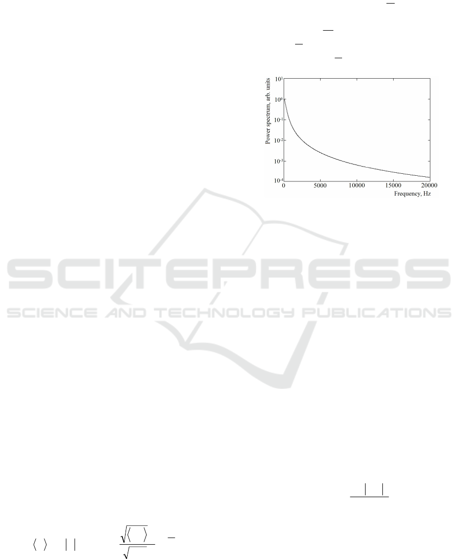
Figure 1: The typical power spectrum P(ω) of the laser
Doppler signal described by the B&N model.
Surprisingly, in (1) there is not any dependence
on the wavelength λ
0
of probing radiation, i.e. the
waveband of the phenomenon doesn't matter...
3 BACKGROUND OF THE FIRST
PRINCIPLES
Since almost all modern diagnostic optics and
electronic devices are constructed nowadays as
analog-to-digital measuring systems, in most cases
an analyzed signal is a voltage u(t) as a function of
time. Often u(t) is formed at the input of measuring
converter, for example, at the input of the analog-
to-digital converter, as a voltage drop on the
measuring resistance R
m
due to a photocurrent flow
through the R
m
. This photocurrent i(t), in its turn, is
proportional to the squared modulus of the optical
field |E(t)|
2
incident on a photodetector due to a
quadraticity nature of the photodetection:
e
Z
ti
2
E(t)A
~)(
2

, (2)
where η is a conversion factor of the photodetector
(A/W); A is a surface area of the photodetector
(m
2
); E(t) is the electric field of radiation (V/m); Z
e
is the wave impedance of the medium (Ohm).
The spectrum (spectral density) of the measured
signal u(t)=R
m
·i(t) is determined from (2) by the
spectral density of the intensity |E(t)|
2
, which can be
New Simple Phenomenological Model for Laser Doppler Measurements of Blood Flow in Tissue
99

calculated using the direct Fourier transform:




 dteG
tj
E
2
E(t))(
, (3)
where G(ω) is a spectral density and ω is the
angular frequency of the |E(t)|
2
fluctuations.
If heterodyne mixing of two harmonic waves on
a photodetector is considered, then:
tj
tj
eEeEtE
10
10
)(



, (4)
where ω
0
and ω
1
are frequencies of the waves, E
0
and E
1
are amplitudes of their fields. In this case,
the photocurrent classically can be computed as:
tEEEEti )cos(2E(t)~)(
0110
2
1
2
0
2
 
. (5)
Besides of the constant component with the
amplitude A
0
=E
0
2
+E
1
2
, this mixed signal has the
LFF with the amplitude of fluctuations A
1
=2E
0
E
1
at
the difference frequency ω
d
=(ω
1
–ω
0
), which are
formed due to the beating effect of two fields. Thus,
the spectral density of |E(t)|
2
will have the form:
)(2)()()(
10
2
1
2
0 dE
EEEEG 
, (6)
where δ(x) is the delta function. In the case of light
scattering on a stationary tissue matrix and on the
moving RBCs, ω
d
represents the Doppler frequency
shift. This G
E
(ω) is a discrete (a line) spectrum of
two lines:
)(2)(
)()()(
101
2
1
2
00
dE
E
EEG
EEG


(7)
with amplitudes of lines A
0
and A
1
, which are
determined by integration of (7) over ω. This well-
known result was obtained at the assumption of a
coherence (inphase) of the registered fields. The
less the coherence degree of fields the less the
beating amplitudes are observed. As to LDF, the
light scattering in tissues is a random process over
its volume. So, the phase shift of all mixed waves
will be partially random, and (6) should be rewritten
taking into account the coherence coefficient ξ
0,1
of
these two waves (Born and Wolf, 1964):
tEEEE
d
 cos2E(t)
101,0
2
1
2
0
2

, (8)
where 0 ≤ ξ
0,1
≤ 1. Similarly, if the sum of three or
even more fields with frequencies ω
0
; ω
1
; ... ω
n
is
considered, where each frequency ω
k
=ω
0
+ω
dk
(k=1,
2, 3 … n), then:



n
k
kkk
n
k
k
tEEE
1
0,00
0
2
2
)cos(2E(t) 
(9)





n
jk
kjkkj
n
j
j
tEE
1
,
1
1
)cos(2 
Without the loss of generality, we may accept
for further analysis ξ
0,k
=const=ξ. Since for LDF all
E
k
at k>0 are the field amplitudes scattered by
RBCs, then coefficients of their mutual coherence
ξ
m,k
at m≠0 are ξ
m,k
<<ξ
0,k
because the correlation
between reference and scattered fields always is
higher than the correlation between two randomly
scattered fields. It is obvious, also, that E
k
<<E
0
at
k≠0 because a fraction of RBCs in tissues is much
less than a fraction of the tissue matrix. Thus, with a
high degree of accuracy we may retain only first
two sums in the equation (9). It yields:



n
k
dkk
n
k
k
tEEE
1
0
0
2
2
cos2E(t) 
. (10)
In analogy with (3)-(8), the spectral density of
the registered signal (10) will consist of a series of
“k” lines, which spectral amplitudes A
k
at
frequencies ω=ω
dk
for k >0 are:
kk
EEA
0
2


. (11)
Equations (10)-(11) allow one to obtain the spectral
density of the registered signal if all A
k
are known.
4 EVALUATION OF SPECTRAL
AMPLITUDES
Analytical estimation of the amplitudes A
k
is always
preferable. For this purpose, the improved two-flux
Kubelka-Munk model is a good tool (Lapitan et al.,
2016). To obtain the general qualitative result, the
homogenous tissue model in the form of a semi-
infinite turbid medium filled with blood can be
used. The absorption coefficient μ
a
as well as the
average density μ
ρ
of scattering inhomogeneities
inside the tissue can be written as follows:
babata
C





;
bbt
C



, (12)
where μ
at
and μ
ab
are absorption coefficients of a
bloodless tissue and a blood, μ
ρt
and μ
ρb
are the
average density of scatterers inside the bloodless
tissue and the blood respectively, C
b
is a relative
fraction (C
b
=0…1) of the blood in tissues. In (12) it
is assumed, that the volume of blood in tissues is
much less than the volume of the tissue matrix.
For LDF it is sufficient to consider only the
single scattering approximation (SSA). The
intensity of a backscattered flux for SSA and for the
semi-infinite turbid medium can be written as
follows (Dmitriev et al., 2004):
)2exp()1(1
)exp(
0




a
a
BS
R
RF
I



, (13)
where R is a reflection Fresnel coefficient on
borders of inhomogeneities inside the medium, F
0
–
incident flux. Since C
b
<1 and usually |μ
a
/μ
ρ
|˂˂1,
together with (12) the equation (13) can be
expanded in a Taylor series by μ
a
/μ
ρ
and C
b
. After
BIODEVICES 2017 - 10th International Conference on Biomedical Electronics and Devices
100

transformations, living only two first terms, one will
have:

























b
t
ab
t
bat
BS
CZYI
2
1
, (14)
where:
WWZ /)2( 
;
)2exp()1(1
tat
RW

 
and
WRFY
tat
/)exp(
0 
 
.
The total backscattered radiation incident on a
photodetector is the mixed radiation:
dBS
III 

0
, (15)
where I
0
is the intensity of the scattered flux without
Doppler shift and I
d
is the intensity of the Doppler-
shifted flux scattered on moving RBCs. For SSA, I
0
can be determined from (14) at C
b
≠0, μ
ab
≠0, μ
ρb
=0:




















 b
t
ab
bBS
CZYII 1)0(
0
. (16)
Then, I
d
can be determined as follows:
b
t
bat
bBSd
CYZIII
2
0
)0(







. (17)
If different groups of RBCs have different
speeds V
k
(k =1, 2...n), then for each k-th fraction
C
bk
of RBCs its Doppler-shifted flux can be written
as:
bk
t
bat
dk
CYZI
2





. (18)
Note, that



n
k
dkd
II
1
, as well as



n
k
bkb
CC
1
are
conditions closing the distribution. If the discrete
velocity distribution of RBCs is proposed, then all
fluctuation amplitudes A
k
at frequencies ω
dk
can be
computed easily with the use of (10)-(18):
bk
t
bat
b
t
ab
k
CYZCZYA
2
12~
















. (19)
From (19) it follows exactly, that A
k
depend on
ω
dk
like the distribution of
bk
C
, because other
multipliers in (19) are independent on ω
dk
.
5 EVALUATION OF
CONTINUOUS SPECTRA
Usually in LDF, a continuous distribution of RBCs’
velocities such as Maxwell’s distribution is used:
dVV
V
VdF
V
V
)2exp(
2
)(
22
3
2



, (20)
where V is the RBCs velocity, σ
V
is r.m.s. deviation
of V. The density of this distribution has the form:
)2exp(
2
)(
22
3
2
V
V
V
V
Vf 


. (21)
It also can be expressed with the use of the most
probable value V
m
of the velocity:
Vm
V  2
, (22)
or with the use of the most expected mean value of
the velocity <V>:





mV
V
V
222
. (23)
However, we need to have the Doppler-shift
frequency distribution for RBCs, not the
distribution of their velocities. To obtain one it is
necessary to substitute in (20) a value of ω
dk
instead
of V. In the case of SSA, we can use the well-
known expression:
d
V 



4
0
, (24)
It should be also taking into consideration that:
d
ddV 


4
0

. (25)
As a result, omitting the index "d" and taking into
account (23), the distribution density of the Doppler
frequency shift will get the form:
)4exp(
2
)(
2
322
0
3
5
23
0
V
V
f 



. (26)
Each specific C
bk
*
for the frequency interval Δω
k
is determined then from (26) by the integration:




k
dfCC
bbk
)(
(27)
If the density function f(ω) for C
bk
is known,
then it is possible to compute the distribution
density for
bk
C
- the function f’(ω) (see
Appendix A):
)4exp()(
2
342
0
3
5
53
0
V
V
f 




. (28)
Thus, the dependence of spectral amplitudes A
k
on the frequency ω in the case of a continuous
speed distribution gives the spectral density G(ω):
)4exp(~)(
2
342
0
3
5
53
0
V
V
G 



. (29)
We should understand (29) in such a way, that it
reflects qualitatively a spectrum of the photocurrent
LFFs (ac part of i(t)). The function f’(ω), which
determines G(ω) (29), is shown in Figure 2. There
is a series of curves for different <V> in the typical
range of practical relevance of <V>=0,02...1,5 mm/s
at λ
0
=810 nm. In addition, the approximating
exponential function (black dotted line) as well as
New Simple Phenomenological Model for Laser Doppler Measurements of Blood Flow in Tissue
101

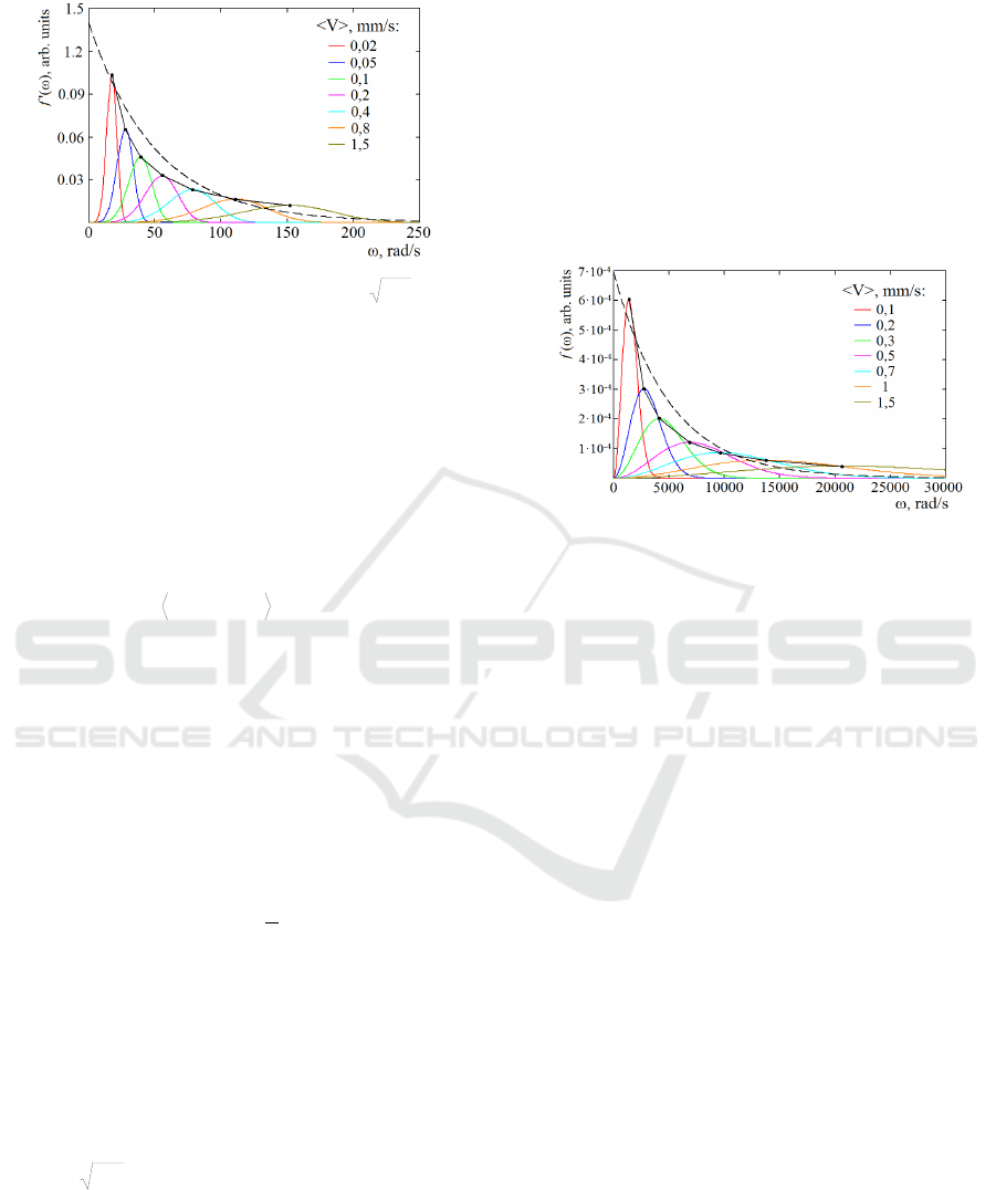
1/ω function (black solid line) are presented.
Figure 2: Distribution density f’(ω) for
bk
C
as a
function of the mean velocity <V> of RBCs (colored
curves), approximating exponential function (black dotted
line) and approximated 1/ω function (black solid line).
Approximating exponential function for (28) is:
)02,0exp(14,0)(
'
 
a
f
. (30)
It should be specially noted, that in the known
B&N model the photocurrent spectrum (29) was not
considered. All classic approaches considered the
autocorrelation function for the photocurrent:





detitiP
j
)()()(
, (31)
which is of the order of the squared photocurrent
i
2
(t) and reflects its power spectrum. To register
i
2
(t), the quadratic converter in the instrument is
required. To compute P(ω) in our approach, it is
necessary to take into consideration, that:
2
1
2
0
22
cos4~)(









n
k
dkk
tEEti
. (32)
As a result, we will have three terms for i
2
(t) due
to the strict phase synchronism of all components:




n
k
dkk
n
k
dkk
tEtE
1
2
1
22
1
2cos1
2
1
cos
,
(33a)





n
k
dmdk
n
km
mk
tEE
1
1
1
2
)cos(
, (33b)





n
k
dmdk
n
km
mk
tEE
1
1
1
3
)cos(
. (33c)
In this case, P(ω) will be determined by the
distribution of C
bk
(26), because each E
k
and E
m
includes
bk
C
, and when multiplying they will give
C
bk
. Herewith, the cosines of close frequencies in
(33b) in the limit to the continuous spectrum will be
approximately equal to 1. The cosines of close
frequencies in (33c) will give the doubled frequency
and will become comparable with terms in (33a),
allowing us to summarize them. The remaining
components will be significantly less than the
enhanced sum (33a), so for a qualitative analysis
they can be neglected without the loss of the
accuracy. Thus, the amplitude-frequency properties
of i
2
(t) are mainly defined by Maxwell’s frequency
distribution (26), but with twice-shifted frequencies
upwards due to squared cosines.
The distribution density f(ω) for C
bk
, which
determines P(ω), is shown in Figure 3. For P(ω) the
approximating exponential function is:
)0002,0exp(0007,0)(
''
 
a
f
. (34)
Figure 3: Distribution density f(ω) for C
bk
as a function of
the mean velocity <V> of RBCs (colored curves),
approximating exponential function (black dotted line)
and approximated 1/ω function (black solid line).
6 DISCUSSION AND
CONCLUSIONS
In this study, we have attempted to propose a new
approach in LDF theory. From “first principles” of
the classic spectral analysis, using the simplest SSA
to determine the intensity of backscattered
radiation, as well as with the use of the Maxwell’s
velocity distribution for moving RBCs, we have
obtained the similar result as it was presented by
Bonner and Nossal. For example, we have obtained
the same order of the waveband of the summarized
power spectrum P(ω) for the squared photocurrent
i
2
(t) (Figure 3), but in a more simple way. What
also is interesting in our result - the approximation
function for P(ω) has the exponent power of
0,0002ω, exactly as it was stated in the end of the
article (Koelink et al., 1994). Moreover, unlike the
B&N model, we have obtained the spectral density
of the photocurrent G(ω), as well. It has the main
spectral region in a low-frequency waveband
(Figure 2), exactly where the LFF of the LDF signal
are often observed. Is there in other publications
such spectra? We have found the same spectra in
the article on a portable Laser Doppler Flowmeter
(Hu et al., 2013). It contains the spectrum of the
BIODEVICES 2017 - 10th International Conference on Biomedical Electronics and Devices
102

same order of the waveband. Determining the
spectrum, authors used i(t), so our theoretical result
is in a good correlation with their experimental one.
And, at last, in contrast to the B&N equation (1),
in our output the weighted beating frequency <ω>,
which is defined as the first moment of P(ω), can be
analytically derived from (24) as:
0
/4  V
.
We see the linear relationship between <ω> and
<V>, like in the B&N model, but we also see the
inverse proportionality to the λ
0
. The absence of one
in (1) looks not physically explained. Moreover, in
(1) the inverse proportionality of <ω> to the
average radius of scatterers “a” without taking into
account any light diffraction looks not quite
justified, as well. What if in the limit a→0?
Thus, we see several advantages in our
approach. It is a qualitative approach, an
approximation only, but it allows to understand
better several features of the input signal spectral
properties in LDF. For example, it assists to
understand better, that the power spectrum in the
exponential form, similar to a fractal noise, is the
consequence mainly of the Maxwell’s distribution,
not of the specialties of light scattering in tissues.
Additionally, at SSA the linear proportionality
between <ω> and <V> is a trivial consequence of
the Doppler effect, (24) not more.
REFERENCES
Bonner, R. and Nossal, R., 1981. Model for laser Doppler
measurement of blood flow in tissue. Applied Optics,
20(12), 2097-2107.
Born, M., Wolf, E., 1964. Principles of optics. Second ed.
Pergamon press, Oxford-London-Edinburgh-Paris.
Cummins, H.Z. and Swinney, H.L., 1970. Light Beating
Spectroscopy. Progress in Optics, 8, 133-200.
Dmitriev, M.A., Feducova, M.V., Rogatkin, D.A., 2004.
On one simple backscattering task of the general light
scattering theory. Proc. SPIE., 5475, 115–122.
Hu, C. L., Lin, Z. S., Chen, Y. Y., Lin, Y. H., Li, M. L.,
2013. Portable laser Doppler flowmeter for
microcirculation detection. Biomedical Engineering
Letters, 3(2), 109-114.
Koelink, M.H., De Mul, F.F.M., Leerkotte, B., et al.,
1994. Signal processing for a laser-Doppler blood
perfusion meter. Signal processing, 38(2), 239-252.
Lapitan, D.G., Rogatkin, D.A., 2016. Variable hyperemia
of biological tissue as a noise source in the input
optical signal of a medical laser Doppler flowmeter.
J. Opt. Techn., 83(1), 36-42.
Mizeva, I., Maria, C., Frick, P., Podtaev, S., Allen, J.,
2015. Quantifying the correlation between
photoplethysmography and laser Doppler flowmetry
microvascular low-frequency oscillations. J. of
Biomed. Optics, 20(3), 037007.
Mizeva, I., Frick, P., Podtaev, S., 2016. Relationship of
oscillating and average components of laser Doppler
flowmetry signal. J. of Biomed. Optics, 21(8),
085002.
Nilsson, G.E., Tenland, T., Oberg, P.A., 1980. A new
instrument for continuous measurement of tissue
blood flow by light beating spectroscopy. IEEE
Transactions on Biomed. Engineering, 27(1), 12-19.
Podtaev, S., Stepanov, R., Smirnova, E., Loran, E., 2015.
Wavelet-analysis of skin temperature oscillations
during local heating for revealing endothelial
dysfunction. Microvascular research, 97, 109-114.
Rajan, V., Varghese, B., Leeuwen, T., 2009. Review of
methodological developments in laser Doppler
flowmetry. Lasers Med Sci, 24, 269–283.
Roustit, M., Cracowski, J., 2012. Non-invasive
assessment of skin microvascular function in humans:
an insight into methods. Microcirculation, 19(1), 47-
64.
Shiryaev, A.N., 1996. Probability. Springer, New York.
APPENDIX A
According to Kolmogorov’s axiomatic, a random variable
is a measurable function on the probability space (Ω,
,ℙ) (Shiryaev, 1996). Let a real random variable




has the probability density

px

. Let a continuous
function of this random variable





f

 
has a
probability density


px

. We are going to prove, that
 


:tf t x
d
p
xptdt
dx








.
The definition of a distribution function

F
x

of




is:






:Fx
x

 

 . Substituting the
definition of



 , we obtain
  




:Ffx
x

 


. Probability in the right
hand side can be rewritten as an integral of p

over a set
of points in which


f

is not greater than
x
:






:tft x
Fx ptdt




. To find the density

px

it
remains to differentiate


F
x

:
  


:tf t x
dd
p
xFx ptdt
dx dx
 







.*
* Note: The existence of the density

px

is not
guaranteed for all




and

f

. Here, we don’t study
conditions under which the density of



exists, but
we require
its existence.
New Simple Phenomenological Model for Laser Doppler Measurements of Blood Flow in Tissue
103