Bimodal Model-based 3D Vision and Defect Detection for Free-form
Surface Inspection
Christophe Simler, Dirk Berndt and Christian Teutsch
Fraunhofer Institute for Factory Operation and Automation IFF, Sandtorstrasse 22, 39106 Magdeburg, Germany
Keywords: Detection, Inspection, Free-form Surface, Photogrammetry, Photometric Stereo, Shape Analysis,
Model-based, Data Simulation, Merging, Supervised Classification, Image Segmentation.
Abstract: This paper presents a 3D vision sensor and its algorithms aiming at automatically detect a large variety of
defects in the context of industrial surface inspection of free-form metallic pieces of cars. Photometric
stereo (surface normal vectors) and stereo vision (dense 3D point cloud) are combined in order to
respectively detect small and large defects. Free-form surfaces introduce natural edges which cannot be
discriminated from our defects. In order to handle this problem, a background subtraction via measurement
simulation (point cloud and normal vectors) from the CAD model of the object is suggested. This model-
based pre-processing consists in subtracting real and simulated data in order to build two complementary
“difference” images, one from photometric stereo and one from stereo vision, highlighting respectively
small and large defects. These images are processed in parallel by two algorithms, respectively optimized to
detect small and large defects and whose results are merged. These algorithms use geometrical information
via image segmentation and geometrical filtering in a supervised classification scheme of regions.
1 INTRODUCTION
The context of this article is the industrial surface
inspection (defect detection) of free-form metallic
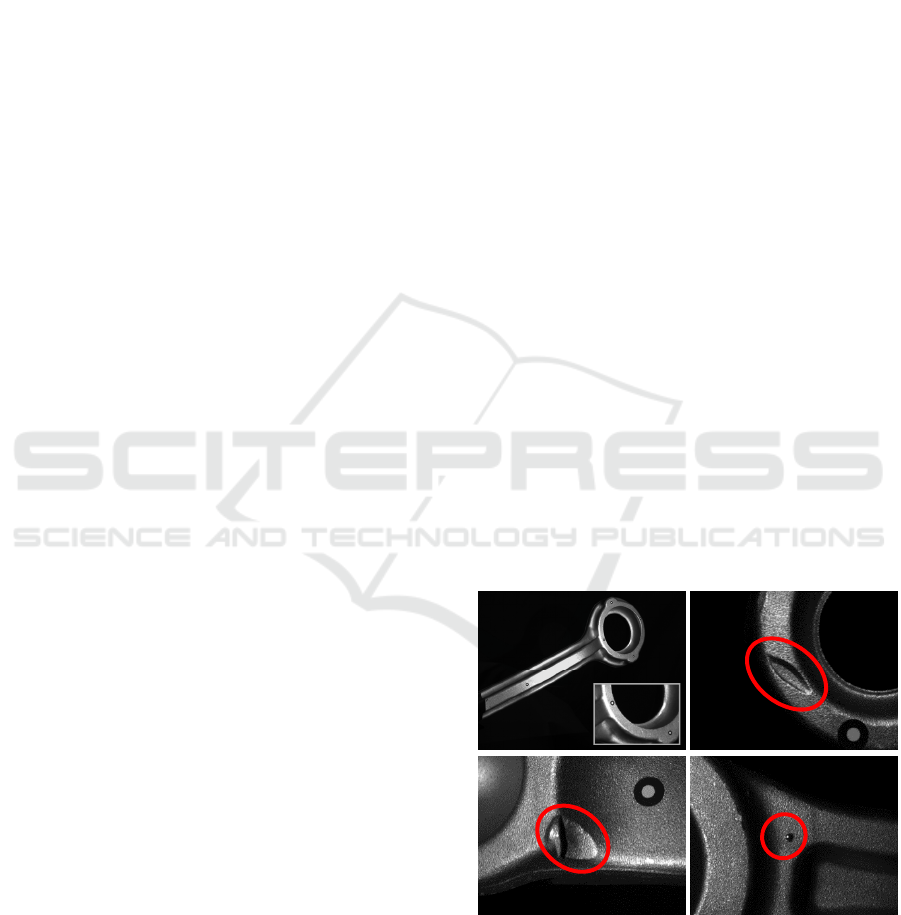
car parts. Such a part is shown at the top left of
figure 1. Inspection is performed just after the
production and is generally done by human experts.
This has the drawbacks to be tiring, costly and above
all subjective. Many efforts are currently done to
automate this process. Comparing to most of the
existing automated inspection procedures, the new
challenge is to handle free-form surfaces.
Standard industrial cameras and controlled
lighting are used in this work. Three examples of
defects visualized by a sensor composed of a camera
(resolution: 33um/pixel) and one punctual light
source are shown on figure 1. Traditionally in
industry, feature extraction and classification are
applied on images of relatively planar surfaces. Such
procedures applied on images of free-form surfaces
will lack of reliability because:
1- Visibility (shading) problem: because of
the free-form of the surface, the visibility of
a defect in the image depends too much on
the positions of light source and camera.
2- Background problem: the free-form of the
surface introduces natural edges which
cannot be easily discriminated from our
“unfeatured” defects.
Figure 1: Top-left: free-form mechanical parts of cars.
Others: examples of defects of different shape and size.
The first problem discards the direct use of such
images as input of the detection algorithm. Because
our defects are 3D, a solution is to use 3D vision
sensors. We use photometric stereo (building an
Simler C., Berndt D. and Teutsch C.
Bimodal Model-based 3D Vision and Defect Detection for Free-form Surface Inspection.
DOI: 10.5220/0006113304510458
In Proceedings of the 12th International Joint Conference on Computer Vision, Imaging and Computer Graphics Theory and Applications (VISIGRAPP 2017), pages 451-458
ISBN: 978-989-758-225-7
Copyright
c
2017 by SCITEPRESS – Science and Technology Publications, Lda. All rights reserved
451
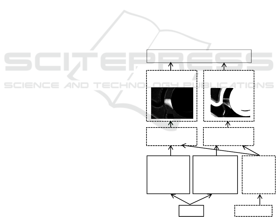
image of surface normal vectors), avoiding the
shading problem and enabling the detection of our
“small” defects. However, it is only sensitive to the
defect depth gradient and its integration lacks of
reliability (Ne, 05). This limits the ability to detect
some of our flat “large” defects, such as the one at
the top right of figure 1. To overcome this problem,
an active stereo vision system (building a dense 3D
point cloud) is also used.
The second problem occurs whatever the data
used, and thus a pre-processing has to be done.
Some methods currently applied on images could be
applied on 3D data. Thus they are presented below
although only 3D data are used in our work. There
are two approaches suggested in the literature to
solve the second problem: restoration and
background subtraction.
Restoration: it filters the undesired elements. It is
used in inspection of textile, wood and metallic
surfaces to remove structural/statistical textures (Ts,
01) (Ts, 03), or repetitive patterns (He, 05) in which
the defect is embedded. Morphological filters are
also used to highlight defects of specific shapes (Zh,
02). However, natural edges have no specific
features and cannot be discriminated from our
defects, thus they cannot be filtered.
Background subtraction (applied on images and
3D data): it consists of building a (monochrome)
“difference” image (input of the classification
algorithm) by subtracting a reference data set (our
“background” is the data without defect) from the
real data set. In the difference image, the defect
generally contrasts in radiometry with the
background. In the context of change or motion
detection in images, the reference data set is often an
image of the same scene taken previously. In our
context it has to be built. In (Ch, 16), the theory of
sparse representation and dictionary learning is used
in the case of images. This approach generates a
“flexible” reference image, adjusted to the
uncertainties (localization, illumination, texture and
geometric tolerances of the part) of its corresponding
real image. The success of the method depends on
the reliability of the decomposition models and on
the quality of the dictionary, which is generally
learned (Lu, 13). However, the method has not been
yet extended to 3D data, and this is why we do not
use it in this work.
Another technic to obtain a reference data set is to
simulate the data from the CAD object model. To
perform that, we have developed a simulator
enabling to work in a 3D virtual space containing the
CAD and the sensor model. The sensor model can
be moved with respect to the CAD, and sensor data
can be simulated from a chosen viewpoint. In our
application, once the real sensor is localized with
respect to the object, the sensor model is positioned
accordingly in the virtual space in order to obtain
simulated data registered with the real data. This
model-based approach generates a “perfect”
reference data set, but not a “flexible” one like with
a dictionary. However, it has the great advantage to
be easily used with 3D data, and this is why we use
it in this work. In our context of image-based defect
detection, the CAD model is currently not very used
in industry, and when it is used it is generally
without data simulation.
In this work two 3D vision sensors are used (for
large and small defects). For each one, a model-
based background subtraction generates a difference
image. The independent and complementary
“photogrammetric” and “photometric” difference
images are the input of the classification algorithm
(see figure 2). Figure 3 shows the hardware of the
system. (Ne, 05) suggests a rendering technic
building an “improved” 3D point cloud by
combining a measured 3D point cloud and a surface
normal vector image. Data merging presenting a risk
of loss of information, it is not retained in this work.
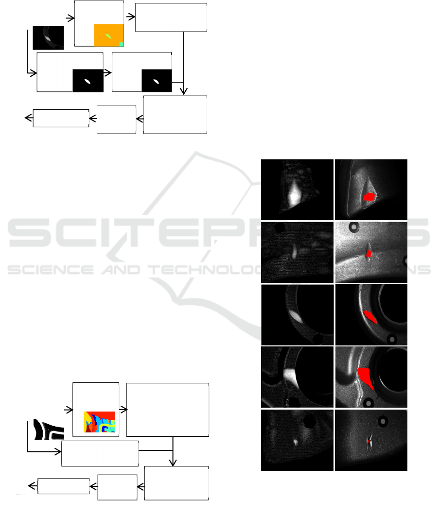
Figure 2: Flow diagram of the defect detection system: 3D
vision sensor combination (solid boxes), background
subtraction via simulation from the CAD model (dotted
boxes), and finally feature extraction, classification,
merging and decision algorithm.
Photogrammetric
difference image
Photometric
difference image
Defect detection algorithm and decision
Simulated
data (ref.)
via sensor
models
(
localize
d
Real data:
surface normal
vector image
from photome-
tric stereo
CAD model
Real data:
dense 3D
point cloud
from active
stereo vision
Ob
j
ect
Background
subtraction
Background
subtraction
VISAPP 2017 - International Conference on Computer Vision Theory and Applications
452

Figure 3: Hardware of the vision system (fully-calibrated).
The sensors and their ability to visualize defects in
their difference images are explicated in part 2. The
classification algorithm (and related works) is
detailed in part 3. The classification results are in
part 4 and part 5 is the conclusion.
2 SENSORS & VISUALIZATION
This section presents our two 3D vision sensors and
shows their complementarity and ability to visualize
defects in their difference images. The first sensor
uses photometry to visualize small defects (their
gradients are visualized), while the second uses
photogrammetry for visualizing large defects.
2.1 Photometry
The resolution of our camera is 33um/pixel,
enabling to visualize our small defects, which can be
as small as 0.3mm². Photometric stereo (building an
image of surface normal vectors) provides a
difference image of this resolution while avoiding
shading effect. The difference image visualizes the
defect depth gradient.
Photometric stereo consists in reconstructing the
surface normal vectors from N images N 3
having different illuminations. Let us consider the
case of a perfectly diffuse surface (Lambertian
reflectance model). For each pixel we have N
brightness equations: I
I
ρv
.n with 1 i
N. I
are the measured pixel intensities. v
and
I
are the (generally known) light source
directions (vectors) and intensities. n is the
(normalized) surface normal vector and ρ is the
surface albedo (generally unknown). Thus we have
N non-linear equations and three unknowns. This
system has a closed-form solution. See (He, 11) for
generalization.
Photometric stereo in our work and contributions:
our sensor contains eight distant and punctual light
sources (figure 3). We assume that our surface
reflectance has diffuse and specular components.
Also, our free-form surface and the 3D defects
produce shadows in the images. Thus, the i
intensity of a pixel in our sequence is not
systematically close to I
ρv
.n (Lambertian model),
but can be clearer due to specularity or darker due to
shadow. We discard these outliers using the method
of (Br, 12) and then estimate the normalized surface
normal vector and the albedo from (at least three)
inliers via least squares. Our contribution is that we
overcome the problem of the limited dynamic range
in intensity of the camera. For each illumination, a
robust high dynamic range (HDR) image is
computed from five acquisitions with different
exposure times (He, 14).
Our photometric stereo sensor provides a “color”
image containing the normalized surface normal
vectors (see figure 4.1, figure 6.1 is the raw image).
The difference image is formed with the Euclidian
distances between these real vectors and their
corresponding simulated ones (simulation in figure
4.2; difference image in figure 4.3). The intensity of
this image is related to the absolute value of the
defect depth gradient. Figure 5.1 shows a zoom of a
small defect (kind of dome). Without surprise, its
depth gradient is visible in the difference image
(figure 5.2). Photometric stereo is a gradient
measurement, and it is difficult to reconstruct the
defect depth by integration. Thus this approach has
difficulties to visualize properly large defects having
flat surfaces (missing material). An example is
shown on figure 4.3 (raw image on figure 6.1). To
overcome this problem, stereo vision is combined
with photometric stereo (part 2.2).
Figure 4: 1: Real (normalized) surface normal vector
image. 2: Simulated data. 3: “Photometric” difference
image (defect depth gradient are visible).
2
Background subtraction (pixel color vector distance)
1
fringe
projector
and camera
for active
stereo vision
Light
sources for
photometric
stereo
Central camera for
photometric stereo
3
Bimodal Model-based 3D Vision and Defect Detection for Free-form Surface Inspection
453
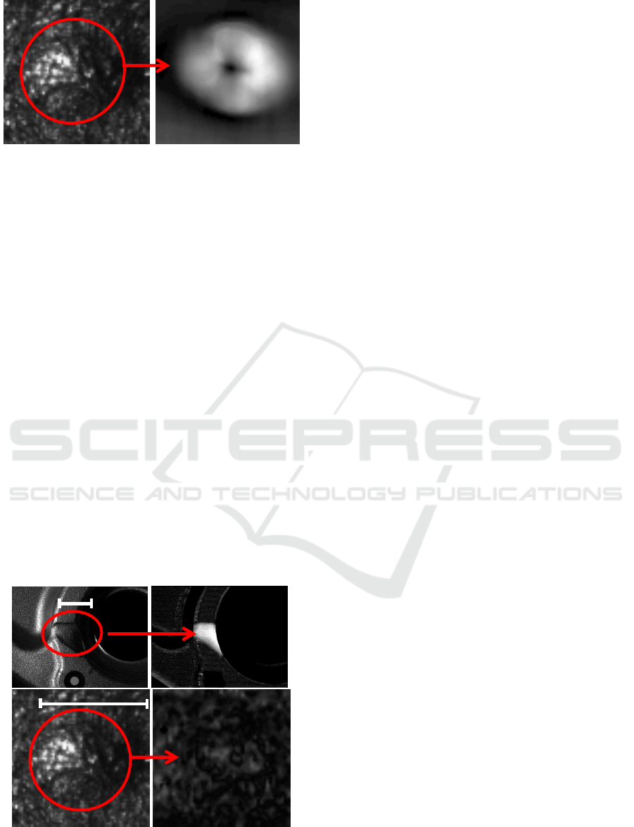
Figure 5: 1: Zoom of a small defect such as the one at the
bottom right of figure 1 (dome of area 0.8mm²). 2:
“Photometric” difference image.
2.2 Photogrammetry
Because photometric stereo is limited to visualize
large defects, this part introduces an active stereo
vision system (producing a dense 3D point cloud)
enabling their suitable visualization. The difference
image is formed with the Euclidian distances
between the real 3D points and their closest
simulated ones. The intensity of this image is related
to the absolute value of the defect depth. Without
surprise, large and deep defects are very visible with
photogrammetry (see figure 6.2; figure 6.1 is the raw
image), and the visibility is much better than with
photometry (compare figure 6.2 with figure 4.3).
The resolution of the “photogrammetric” difference
image is only of 0.9mm² (triangulation-based
methods generally provide a resolution loss (He,
11)). In fact, our stereo vision system cannot
visualize our smallest defects (figures 6.4). This is
not important because the photometric stereo system
handles the small defects (figure 5.2), but shows the
complementarity of the two systems.
Figure 6: 1: a large defect, 3: same as figure 5.1. 2 and 4:
“photogrammetric” difference images.
3 DETECTION ALGORITHMS
Automated and reliable defect detection algorithms
for the inspection of mechanical parts are more and
more needed in industry. Section 3.1 briefly presents
the main classification technics in image processing,
and positions our work with respect to them. Section
3.2 describes our defect detection algorithm.
3.1 Brief Background and Position of
our Method
Some detection algorithms are directly applied to 3D
measured data (Th, 15). However in the following
only image classification is considered, because our
detection algorithm has images in input (the
monochrome difference images). A classification
approach is characterized by the entities it considers
(pixels or objects), the feature extraction and the
classifier itself.
Whatever the context, the most used approach is
by far the classification of pixel features (intensity,
RGB vector …) (Lu, 14) (Ts, 03) (Zh, 02) and (Ch,
16). This approach is used in the article (Li, 07)
using the Torrance and Sparrow surface reflectance
model parameters (computed from photometric
stereo) as pixel features. However, with this technic
each pixel is processed individually without
considering its spatial context in the image (no
overall regularization). Pixel-wise classification is
not used in our work because it can provide a
relative instability (our defects are objects, not
pixels) and does not use any spatial information.
Approaches based on hidden Markov random fields
exploit spatial information (Sc, 09). The problem is
that they require initialization and are time
consuming when large images are processed.
Image segmentation avoids the previous
drawbacks and uses contextual information in order
to group pixels into objects (regions) (Ta, 10) (De,
09). In our work, a segmentation algorithm is
applied on the input image (a defect region should
contain at least one segmented object). Once image
segmentation is performed, two strategies can be
used for the classification.
The first is a pixel spectral classification and to
assign to a segmented object the predominant pixel
class within it (majority vote) (Li, 07). This method
does not use geometry, thus it is adequate when the
defects have few specific geometry or e.g. to detect
forests in aerial rural images.
The second is to design and classify a pattern for
the segmented object. When the defects have few
specific geometry (or in natural environment), the
1
2
3
2
1
4
Not visible
1 mm
10 mm
VISAPP 2017 - International Conference on Computer Vision Theory and Applications
454
components of the pattern are generally only spectral
(Li, 07). In man-made environment, classes of
interest often have specific geometry (size, shape)
and in that case the pattern can possibly have
spectral and spatial components. For example, in
order to detect road and building in color (RGB)
aerial urban images, the article (Si, 11) forms a
pattern whose components are the mean RGB vector
over the segmented object (spectral), the area and
the eccentricity (spatial). The use of geometrical
features has improved the class separability and thus
the classification accuracy.
In our work the above second strategy is retained.
However, our defect class has not enough geometric
features to integrate spatial components into the
pattern. In contrast, the defects (or their gradients)
are generally clearer than the background in the
difference images (figure 2). Thus, spectral
components such as the mean intensity value can be
retained. Although (in our work) geometry cannot be
used to form pattern components, it can be exploited
in a soft manner just after the segmentation
(especially for our small defects) in order to
decrease the risk of false positives. If our defect
class has a geometric feature inside a range,
segmented objects outside this range are eliminated.
We call this operation the geometrical filter.
Supervised classification methods (Bi, 07) and
combination of different approaches are intensively
used to detect defects. For example, the article (Su,
08) combines neural network (NN) and fuzzy logic
in order to train a 6-class classifier. In this article,
object-based feature extraction is implicit because
the input image contains only the inspected part on a
perfectly dark background. In the context of road
and building extraction in color aerial urban images,
(Si, 10) combines a “3 class” support vector machine
(SVM) classifier with a single class SVM in order to
improve the classification accuracy.
In our work, the classification is supervised (via a
training set). However, sophisticated supervised
classification schemes such as NN or SVM are not
needed because our pattern has only one (spectral)
component and we have only two classes (defect or
not). Instead, during the learning the threshold is
manually fixed using a training set.
3.2 Our Detection Approach
Figure 7 shows that the two difference images are
processed in parallel by the algorithms algo3D and
algoN, optimized to detect large and small defects
and the results merged with a logical “or”.
Figure: 7: Defect detection algorithm and decision.
Algorithms algo3D and algoN have the same
structure as discussed in the previous section. The
input image is first segmented (object approach),
then a geometrical filter is applied to discard
improbable regions (against false positives).
Afterwards, a one dimensional radiometric pattern is
computed for each (remaining) segmented object.
Pattern classification is performed via a threshold
which was manually fixed using a training set
(supervised classification). It has been noticed that
when a defect area is larger than 5mm²
photogrammetry should be used, else photometry is
more reliable. Thus 5mm² is the border between
large and small defects.
3.2.1 algo3D
This algorithm, described on figure 8, is designed to
detect large defects (from 5 to 200mm²). These
defects have no shape feature, thus the geometrical
filter only discards segmented regions smaller than
0.9mm² (system resolution). The lower limit is
largely smaller than 5mm² because a segmented
region on the defect can be smaller than the defect.
A large defect has generally a depth upper than
0.3mm. A threshold of this value is applied on the
difference image, enabling to form a pattern
invariant with respect to the defect depth: the
number of white pixels in a segmented region
divided by the region area. It also generally discards
almost all the small aggregates produced by the
imperfections of the fringe projector (see figure 10,
left column). The morphological dilatation makes
more compact the large defect regions (suppression
of the holes), while the erosion limits the risk of
false positives by eliminating the possible remaining
bright (above the threshold) small aggregates.
Photogrammetric
difference image
Photometric
difference image
Defect or not
algo3D algoN
Merging
Bimodal Model-based 3D Vision and Defect Detection for Free-form Surface Inspection
455
The lower limit of the geometrical filter enables
the detection of small defects which are larger than
0.9 mm²; however the morphological erosion
reduces this ability. In fact, Algo3D can detect some
small defects but is not optimized for that. In this
case algoN is more performant to detect them.
Figure 8: algo3D: large defect detection from the
photogrammetric difference image.
3.2.2 algoN
This algorithm, described on figure 9, is designed to
detect small defects (from 0.3 to 5mm²). It is the
defect’s gradients which are visible in the
photometric difference image, thus it is these regions
(or part of them) which can be detected instead of
the defect directly. Our small defects have rough
shape features, and thus also the segmented regions
lying on their gradients. They are never extremely
elongated and have no chaotic border. More
precisely, their areas, eccentricities, compactness
and concavities are inside some ranges (see the
geometrical filter in figure 9).
A Canny edge detector is applied to the
difference image to form a pattern invariant to the
defect depth: the percentage of edges in a segmented
region (notably defect’s gradient regions).
Figure 9: algoN: small defect detection from the
photometric difference image.
4 RESULTS
4.1 Qualitative Results
Figures 10, 11 and 12 show large and small defects
respectively detected by algo3D and algoN. The
difference image is at the left, the defect is shown at
the right and the segmented region of the highest
pattern (classified here as defect) is marked in red.
Sometimes the segmented region is spread over
the entire defect (or defect’s gradient), and
sometimes only on a part of it. This mainly happens
when the defect has strong depth only on a part of it
(and also only the segmented region of the highest
pattern is visualized, while possibly some others are
on the defect region and are classified as defect).
The two cases are equivalent because our aim is the
detection, not the accurate extraction. Among these
examples, no defect has been detected by both
algo3D and algoN (complementarity).
Figure 10: Large defects detected by algo3D. Left:
photogrammetric difference image. Right: the segmented
region of the highest pattern (classified as defect) is in red
on the raw image.
Threshold: 0.35
(learned via training set)
Photogrammetric
difference image
Defect
or not
Segmentation
(regions)
Region patterns
(number of white
pixels / area)
Highest
pattern
Classification
Threshold: 0.3mm
Morphological
filter
Geometrical filter
0.9<area<200mm²
Defect
or not
Geometrical filter
0.1 < area < 5mm²
eccentricity > 0.98
12.5<compactness<37
0.9 < concavity
Canny edge detector
(binary image)
Threshold: 0.082
(learned via training set)
Region patterns
(number of edge
pixels / area)
Highest
pattern
Classification
Photometric
difference image
Segmentation
(regions)
VISAPP 2017 - International Conference on Computer Vision Theory and Applications
456
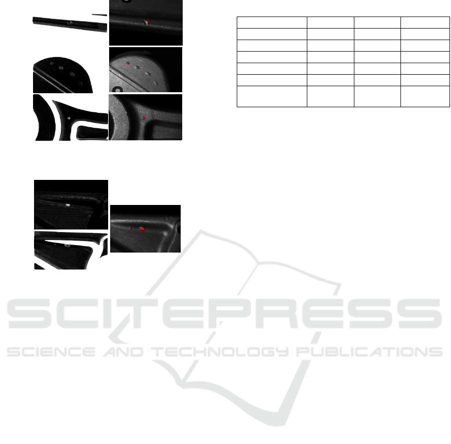
Figure 11: Small defects detected by algoN. Left:
photometric difference image. Right: like in figure 10.
Figure 12: Large and small defects respectively detected
by algo3D and algoN. Left: the photogrammetric (top) and
the photometric (bottom) difference images. Right: like in
figure 10.
4.2 Quantitative Results
Three hundred and sixty five acquisitions are used
for the test. This set includes one hundred and sixty
positives (containing at least one defect), with the
same overall quantity of large and small defects.
Consider algo3D (or equivalently algoN), the
highest pattern and its segmented region:
If the real class is positive: if the segmented
region is on the defect region and the pattern is
classified as positive, we have a true positive (TP). If
the pattern is classified as negative, we have a false
negative (FN). If the segmented region is outside the
defect region and the pattern is classified as positive,
we have a false positive (called FP2).
If the real class is negative: if the pattern is
classified as positive, we have a false positive
(called FP1). If the pattern is classified as negative,
we have a true negative (TN).
The overall accuracy (% of correct
classification) is: 100 /
1 2 . The results of each method are
reported in table 1.
Table 1: Results of the algorithms.
algo3D algoN Merging
TP 112 48 133
TN 205 200 200
FP1 0 5 5
FP2 6 7 6
FN 42 105 21
Overall
accuracy (%)
86.8 67.9 91.2
algo3D provides good results (table 1). As expected,
it detects almost systematically the large defects
(>5mm²), and also sometimes smaller defects. Its
forty two FN are mainly small defects. The results of
algoN are less good. This was expected because it is
designed to detect only small defects. Sometimes
large defects are detected via the detection of parts
of them. More than 80% of the small defects are
detected, this is better than with algo3D. The
combination of these complementary algorithms
significantly improves the overall accuracy with
respect to algo3D. algoN is very useful because it
detects twenty one (generally small) defects that
algo3D not detects. Only twenty seven TP are
detected by both algo3D and algoN. This confirms
their high complementarity.
FP1 and FP2 are due to higher measurement
error at natural edges. These errors are often visible
in the difference images and sometimes detected,
particularly with algoN due to its higher sensitivity.
FN are the main problem because more numerous.
They occur mainly with small defects (algoN).
Generally, the segmentation extracts them suitably
(more exactly parts of their gradients are extracted),
thus the problem is a too low pattern. It happens
when the edges of the defect’s gradient are mainly
outside the segmented regions or when the defect is
not visible enough due to low depth gradient (too
few edges extracted).
5 CONCLUSION
A model based vision sensor and defect detection
algorithm combining stereo vision and photometric
stereo were presented. Measurement simulations via
the CAD model enabled to build two complementary
difference images. One visualizes well large defect
depths, making possible the detection of large
defects. The other makes visible small defect depth
gradients, enabling the detection of small defects.
The combination of the results of the two
complementary detectors enables to obtain an
overall accuracy of 91.2%. A future challenge is to
Bimodal Model-based 3D Vision and Defect Detection for Free-form Surface Inspection
457

reduce measurement error at natural edges (FPs).
FNs occur mainly with small defects and are
generally due to a low pattern. A second version of
algoN configured to detect defects having low depth
gradient could be tested. With this third class of
defects, the geometrical filter range for the area
could be from 0.1 to 2mm². The segmented regions
of the defects (or more exactly of parts of the defect
gradients) are relatively elliptic, thus an additional
shape feature “fit with an ellipse” could be included
in the geometrical filter or maybe even integrated as
spatial component into the pattern. The spectral
component of the pattern should be maintained
because other segmented regions are elliptic. To
have a higher spectral component, the Canny edge
detector should be much more sensitive.
The prototype will be completed to perform an
automatic inspection of the entire object via model-
based sensor planning (Ch, 11) and motion planning
(La, 06) technics. A robot arm will move the object
between two successive acquisitions. In the virtual
space, measurements will be simulated from each
computed viewpoint. Then during the plan execution
in the real world, real measurements will be done
from these viewpoints. Once the entire object is
captured, the defect detection processing can be
applied in parallel to the data of each viewpoint.
REFERENCES
Chen, S., Li., Y., and Kwok., NM., 2011. Active vision in
robotic systems: A survey of recent developments. Int.
Journal of Robotics Research, 30(11), 1343–1377.
LaValle, S., 2006. Planning Algorithms, Cambridge
University Press, ISBN 0-521-86205-1.
Bishop, C., 2007. Pattern recognition and machine
learning, Springer. ISBN: 978-0-387-31073-2.
Simler, C., 2011. An Improved Road and Building
Detector on VHR images. IEEE International
Geoscience and Remote Sensing Symposium.
Simler, C., Beumier, C., 2010. Building and Road
Extraction on Urban VHR Images using SVM
Combinations and Mean Shift Segmentation.
International Conference on Computer Vision Theory
and Applications (VISAPP).
Lu, D., 2004. Change detection techniques. International
Journal of remote sensing, 25(12), 2365-2407.
Scarpa, G. and all, 2009. Hierarchical multiple markov
chain model for unsupervised texture segmentation.
IEEE Trans.on Image Processing 18(8):1830-1843.
Tarabalka and all, 2010. Segmentation and classification
of hyperspectral images using watershed
transformation. Pattern Recognition, 43(7), 2367-
2379.
Debeir, O., Atoui H., Simler, C., 2009. Weakened
Watershed Assembly for Remote Sensing Image
Segmentation and Change Detection. International
Conference on Computer Vision Theory and
Applications (VISAPP).
Herbort, S., Wöhler, C., 2011. An Introduction to Image-
based 3D Surface Reconstruction and a Survey of
Photometric Stereo Methods. 3D Research, 2:4,
03(2011)4.
Nehab, D., Rusinkiewicz, S., Davis, J., Ramamoorthi, R.,
2005. Efficiently combining positions and normals for
precise 3d geometry. SIGGRAPH'05, 24(3), 536-543.
Bringier, B., Bony, A., Khoudeir, M., 2012. Specularity
and shadow detection for the multisource photometric
reconstruction of a textured surface. Journal of the
Optical Society of America A, 29(1), 11-21.
Herbort, S. 2014. 3D Shape Measurement and Reflectance
Analysis for Highly Specular and Interreflection-
Affected Surfaces. Thesis. TUD.
Linden, S., Janz, A., Waske, B., and all., 2007. Classifying
segmented hyperspectral data from a heterogeneous
urban environment using support vector machines. J.
Appl. Remote Sens., 1(1).
Tsai, D., Hsiao, B., 2001. Automatic surface inspection
using wavelet reconstruction. Pattern Recognition, 34,
1285-1305.
Tsai, D., Huang, T., 2003. Automated surface inspection
for statistical textures. IVC, 21(4), 307-323.
Henry, Y., Grantham, K., Pang. S., Michael K., 2005.
Wavelet based methods on patterned fabric defect
detection. Pattern Recognition, 38, 559-576.
Chai, W., Ho, S., Goh, C., 2016. Exploiting sparsity for
image-based object surface anomaly detection.
IEEE
ICASSP.
Lu, C., Shi, J., Jia, J., 2013. Online robust dictionary
learning. IEEE Conference CVPR.
Than, D. and all, 2015. Automatic defect detection and the
estimation of nominal profiles based on spline for free-
form surface parts. IEEE ICAIM.
Su, J., Tarng, Y., 2008. Automated visual inspection for
surface appearance defects of varistors using an
adaptive neuro-fuzzy inference system. The
International Journal of AMT, 25(7), 789-802.
Zheng, H., Kong L., Nahavandi, S., 2002. Automatic
inspection of metallic surface defects using genetic
algorithms. Journal of MPT, 125-126, 427-433.
Lindner, C., Leon, F., 2007. Model-based segmentation of
surfaces using illumination series. IEEE Transactions
on Instrumentation and Measurement, 56(4).
VISAPP 2017 - International Conference on Computer Vision Theory and Applications
458
